MSBRIDGE: OPENSEES PUSHOVER AND EARTHQUAKE ANALYSIS OF MULTI-SPAN BRIDGES - USER MANUAL

Transcription

1 STRUCTURAL SYSTEMS RESEARCH PROJECT Report No. SSRP 16/05 MSBRIDGE: OPENSEES PUSHOVER AND EARTHQUAKE ANALYSIS OF MULTI-SPAN BRIDGES - USER MANUAL by ABDULLAH ALMUTAIRI JINCHI LU AHMED ELGAMAL KEVIN MACKIE Final Report Submitted to the California Department of Transportation (Caltrans) under Contract No. 65A0530. July 2018 Department of Structural Engineering University of California, San Diego La Jolla, California

2 University of California, San Diego Department of Structural Engineering Structural Systems Research Project Report No. SSRP-16/05 MSBridge: OpenSees Pushover and Earthquake Analysis of Multi-span Bridges - User Manual by Abdullah Almutairi Graduate Student Researcher, UC San Diego Jinchi Lu Associate Project Scientist, UC San Diego Ahmed Elgamal Professor of Geotechnical Engineering, UC San Diego Kevin Mackie Associate Professor of Structural Engineering, University of Central Florida Final Report Submitted to the California Department of Transportation under Contract No. 65A0530 Department of Structural Engineering University of California, San Diego La Jolla, California July 2018 ii

3 Technical Report Documentation Page 1. Report No. 2. Government Accession No. 3. Recipient s Catalog No. 4. Title and Subtitle MSBridge: OpenSees Pushover and Earthquake Analysis of Multi-span Bridges - User Manual 5. Report Date July Performing Organization Code 7. Author(s) Abdullah Almutairi, Jinchi Lu, Ahmed Elgamal and Kevin Mackie 9. Performing Organization Name and Address Department of Structural Engineering School of Engineering University of California, San Diego La Jolla, California Performing Organization Report No. UCSD / SSRP-16/ Work Unit No. (TRAIS) 11. Contract or Grant No. 65A Sponsoring Agency Name and Address 13. Type of Report and Period Covered Final Report California Department of Transportation 14. Sponsoring Agency Code Division of Engineering Services th St., MS-9-2/5i 15. Supplementary Sacramento, Notes California Prepared in cooperation with the State of California Department of Transportation. 16. Abstract MSBridge is a PC-based graphical pre- and post-processor (user-interface) for conducting nonlinear Finite Element (FE) studies for multi-span bridge systems. Finite element computations are conducted using OpenSees ( an open source framework developed by the Pacific Earthquake Engineering Research (PEER) Center. The analysis options available in MSBridge include: i) Pushover Analysis; ii) Mode Shape Analysis; iii) 3D Base Input Acceleration Analysis (single and/or multiple); iv) Equivalent Static Analysis (ESA); and v) PBEE Analysis. 17. Key Words Finite Element, Time History Analysis 18. Distribution Statement Unlimited 19. Security Classification (of this report) 20. Security Classification (of this page) 21. No. of Pages 22. Price Unclassified Form DOT F (8-72) Unclassified Reproduction of completed page authorized iii

4 DISCLAIMER This document is disseminated in the interest of information exchange. The contents of this report reflect the views of the authors who are responsible for the facts and accuracy of the data presented herein. The contents do not necessarily reflect the official views or policies of the State of California or the Federal Highway Administration. This publication does not constitute a standard, specification or regulation. This report does not constitute an endorsement by the California Department of Transportation of any product described herein. For individuals with sensory disabilities, this document is available in Braille, large print, audiocassette, or compact disk. To obtain a copy of this document in one of these alternate formats, please contact: Division of Research and Innovation, MS-83, California Department of Transportation, P.O. Box , Sacramento, CA iv

5 ACKNOWLEDGMENTS The research described in this report was primarily supported by the California Department of Transportation (Caltrans) with Dr. Charles Sikorsky as the project manager. Additional funding was provided by the Pacific Earthquake Engineering Research Center (PEER). These supports are most appreciated. In addition, we are grateful for the valuable technical suggestions, comments and contributions provided by Caltrans engineers, particularly Dr. Charles Sikorsky, Dr. Toorak Zokaie, Mr. Yeo (Tony) Yoon, Dr. Mark Mahan, Dr. Anoosh Shamsabadi, and Mr. Steve Mitchell. v

6 ABSTRACT MSBridge is a PC-based graphical pre- and post-processor (user-interface) for conducting nonlinear Finite Element (FE) studies for multi-span bridge systems. Finite element computations are conducted using OpenSees ( an open source framework developed by the Pacific Earthquake Engineering Research (PEER) Center. The analysis options available in MSBridge include: i) Pushover Analysis; ii) Mode Shape Analysis; iii) 3D Base Input Acceleration Analysis (single and/or multiple); iv) Equivalent Static Analysis (ESA); and v) PBEE Analysis. vi

7 TABLE OF CONTENTS DISCLAIMER... IV ACKNOWLEDGMENTS... V ABSTRACT... VI TABLE OF CONTENTS...VII LIST OF FIGURES... XI LIST OF TABLES... XVIII 1 INTRODUCTION Overview What s New in Version Units Coordinate Systems System Requirements Acknowledgments GETTING STARTED Start-Up Interface Menu Bar Model Input Region Finite Element Mesh Region BRIDGE MODEL Spans Straight Bridge Curved Bridge Deck Sections Bentcap Sections Column Cross Sections Cross Section Shapes Cross Section Types Foundation Rigid Base vii

8 3.5.2 Soil Springs Foundation Matrix Abutment Bridge Model Column Heights Column Connection Steel Jackets Advanced Options Deck Hinges Isolation Bearings Skew Angles Mesh Parameters ABUTMENT MODELS Elastic Abutment Model Roller Abutment Model SDC 2004 Abutment Model Longitudinal Response Transverse Response Vertical Response Definition of the SDC 2004 Abutment Model SDC 2010 Sand Abutment Model SDC 2010 Clay Abutment Model ElasticPP-Gap Model HFD Model COLUMN RESPONSES & BRIDGE RESONANCE Bridge Natural Periods Column Gravity Response Column & Abutment Longitudinal Responses Column & Abutment Transverse Responses PUSHOVER & EIGENVALUE ANALYSES Pushover Analysis viii

9 6.1.1 Input Parameters Output for Pushover Analysis Eigenvalue Analysis GROUND SHAKING Definition/specification of input motion ensemble (suite) Available Ground Motions Specifications of Input Motions Rayleigh Damping Save Model and Run Analysis TIME HISTORY AND ENGINEERING DEMANDING PARAMETER OUTPUT Time History Output Quantities Deck Response Time Histories Column Response Profiles Column Response Time Histories Column Response Relationships Abutment Responses Time Histories Soil Spring Responses Time Histories Deck Hinge Responses Time Histories Isolation Bearing Responses Time Histories Deformed Mesh and Animation Maximum Output Quantities EDP Quantities Bridge Peak Accelerations & Displacements for All Motions Maximum Column & Abutment Forces for All Motions EQUIVALENT STATIC ANALYSIS Bridge Longitudinal Direction Bridge Transverse Direction PBEE ANALYSIS (GROUND SHAKING) Theory and Implementation of PBEE Analysis Input Necessary for User-defined PBEE Quantities ix

10 10.3 Definition/specification of PBEE input motion ensemble (suite) Available Ground Motions Specifications of PBEE Input Motions Save Model and Run Analysis PBEE Analysis PBEE Quantities Compute Repair Cost & Time Compute Hazard Curves Compute Disaggregation TIME HISTORY AND PBEE OUTPUT Time History Output Quantities PBEE Output Quantities PBEE Outcomes Repair Cost & Time Hazard Curves Disaggregation x

11 LIST OF FIGURES Fig. 1. Global coordinate system employed in MSBridge... 2 Fig. 2. MSBridge main window... 4 Fig. 3. Menu and submenu bars: a) menu bar; b) menu File; c) menu Execute; d) menu Display; e) menu Report; and f) menu Help... 6 Fig. 4. MSBridge copyright and acknowledgment window... 8 Fig. 5. Available actions in the FE Mesh window... 9 Fig. 6. Model builder buttons Fig. 7. MSBridge main window (bridge model with soil springs and deck hinges included) Fig. 8. Spans Fig. 9. Varied span lengths Fig. 10. Straight bridge with different span lengths Fig. 11. Horizontal alignment Fig. 12. Horizontal and vertical alignments: a) horizontal alignment (plan view); b) vertical alignment (side view) Fig. 13. Vertical alignment Fig. 14. Examples of horizontal curved bridges (horizontal alignment): a) single radius horizontal curve; b) multi-radius horizontal curve; c) horizontal curve connecting to straight parts) Fig. 15. Examples of vertically curved bridges (vertical alignment): a) single slope; b) begin and end slopes; c) multiple slopes; d) mixing slope and zero-slope Fig. 16. Material properties of the bridge deck Fig. 17. Box girder shape employed for the bridge deck Fig. 18. Material properties of the bent cap Fig. 19. Rectangular shape employed for the bent cap Fig. 20. Column properties and available beam-column element types Fig. 21. Definition of linear column Fig. 22. Column Elastic material properties Fig. 23. Column Section properties Fig. 24. Nonlinear Fiber Section window xi

12 Fig. 25. Column nonlinear material properties: a) Steel02 material; b) ReinforcingSteel material; c) Concrete02 material for the core concrete; d) Concrete02 material for the cover material Fig. 26. Column fiber section (based on PEER best modeling practices report, Berry and Eberhard, 2007): a) Circle; b) Octagon; c) Hexagon Fig. 27. OpenSees quadrilateral patch employed for calculating the cover concrete fibers for: a) Octagon; and b) Hexagon cross section Fig. 28. Stress-strain curve for a steel material (default values employed): a) Steel01 (with a strain limit); b) Steel02 (with a strain limit); and c) ReinforcingSteel (with a strain limit) Fig. 29. Stress-strain curve of the core concrete material (default values employed): a) Elastic-No Tension; b) Concrete01; and c) Concrete Fig. 30. Stress-strain curve of the cover concrete material (default values employed): a) Concrete01; and b) Concrete Fig. 31. Moment-curvature response for the column (with default steel and concrete parameters, and the deck weight 2500 kip applied at the column top Fig. 32. User-defined moment curvature Fig. 33. User-defined Tcl script for nonlinear fiber section Fig. 34. Foundation types available in MSBridge Fig. 35. Shaft foundation for abutments and bents Fig. 36. Pile foundation model for abutments Fig. 37. Soil springs Fig. 38. Soil spring calculations based on p-y equations: a) Soft Clay (Matlock); b) Stiff Clay without Free Water (Reese); c) Sand (Reese); d) Liquefied Sand (Rollins) Fig. 39. Soil spring definition window after using the soil spring data calculated based on p-y equations Fig. 40. Sample FE mesh of a bridge model with soil springs included Fig. 41. Local coordination system for the foundation matrix Fig. 42. Foundation matrix for each bent Fig. 43. Definition of an abutment model Fig. 44. Columns xii

13 Fig. 45. Column heights Fig. 46. Column boundary conditions Fig. 47. Bridge configuration: a) general options; b) column layout Fig. 48. Definition of steel jackets Fig. 49. Sketch of steel jacket Fig. 50. Advanced options Fig. 51. Definition of deck hinges Fig. 52. FE mesh of a 4-span model with 2 deck hinges included Fig. 53. OpenSees zerolength elements for deck hinges (plan view) Fig. 54. Definition of isolation bearings Fig. 55. FE mesh of a 4-span bridge model with 2 isolation bearings included on each bent cap Fig. 56. OpenSees zerolength elements for isolation bearings (side view of bent cap cut-plan) Fig. 57. Definition of skew angles Fig. 58. Definition of pilecap mass Fig. 59. Definition of steel jackets Fig. 60. Mesh parameters Fig. 61. Definition of an abutment model Fig. 62. General scheme of the Elastic Abutment Model: a) longitudinal component; b) transverse component; c) vertical component Fig. 63. Definition of the Elastic Abutment Model Fig. 64. Parameters of the Elastic Abutment Model Fig. 65. Longitudinal components of the Elastic Abutment Model in a curved bridge: a) left abutment; b) right abutment Fig. 66. Bridge model with multiple distributed springs and a positive skew angle: a) straight bridge; b) curved bridge Fig. 67. General scheme of the Roller Abutment Model Fig. 68. Selection of the Roller Abutment Model Fig. 69. Longitudinal response of the SDC 2004 Abutment Model: a) general scheme; b) longitudinal response of a bearing pad; c) total longitudinal response xiii

14 Fig. 70. Longitudinal response of the SDC 2004 Abutment Model for a curved bridge with a (positive) skew angle Fig. 71. Transverse response of the SDC 2004 Abutment Model: a) general scheme; b) response of a bearing pad and shear keys (curve with a higher peak value is the shear key response); c) total transverse response Fig. 72. Vertical response of the SDC 2004 Abutment Model: a) general scheme; b) vertical response of a bearing pad; c) total vertical response Fig. 73. Definition of the SDC 2004 Abutment Model: a) main parameters; b) bearing pad properties; c) shear key properties; d) SDC abutment properties; e) embankment properties Fig. 74. Backfill horizontal properties for the SDC 2010 Sand Abutment Model Fig. 75. Backfill horizontal properties of the SDC 2010 Clay Abutment Model Fig. 76. Backfill horizontal properties of the EPP-Gap Abutment Model Fig. 77. Definition of the HFD Abutment Model: a) HFD abutment model; and b) HFD parameters for abutment backfills suggested by Shamsabadi et al. (2007); and c) backfill properties of the HFD Model Fig. 78. Buttons to view column & abutment responses and bridge resonance Fig. 79. Natural periods and frequencies of bridge Fig. 80. Column internal forces and bending moments after application of own weight. 81 Fig. 81. Column longitudinal responses Fig. 82. Abutment longitudinal responses Fig. 83. Column transverse responses Fig. 84. Abutment transverse responses Fig. 85. Pushover analysis option Fig. 86. Load pattern for monotonic pushover analysis Fig. 87. Load pattern for cyclic pushover analysis Fig. 88. User-defined pushover (U-Push) Fig. 89. Column response profiles Fig. 90. Column response time histories Fig. 91. Response relationships for column Fig. 92. Abutment response time histories xiv

15 Fig. 93. Deformed mesh and contour fill Fig. 94. Visualization of Plastic hinges (red dots represent plastic hinges developed) Fig. 95. Steps to perform an Eigenvalue analysis Fig. 96. Sample output for an Eigenvalue analysis for the default bridge model: a) first mode; b) second mode; c) third mode; d) fourth mode; and e) fifth mode Fig. 97. Group shaking analysis Fig. 98. Input motions window Fig. 99. Importing a user-defined motion Fig Time histories and response spectra of individual motion Fig Intensity measures of individual motion Fig Histogram and cumulative distribution for the whole input motion set: a) histogram; b) cumulative distribution Fig Rayleigh damping Fig Simultaneous execution of analyses for multiple motions Fig Parameters for OpenSees analysis Fig Selection of an input motion Fig Deck longitudinal displacement response time histories Fig Displacement profile in the longitudinal plane Fig Bending moment profile in the longitudinal plane Fig Response time histories and profiles for column (and pile shaft): displacement is shown at the nodes Fig Load-displacement curve at column top Fig Moment-curvature curve at column top Fig Abutment longitudinal force-displacement relationship: a) left abutment; and b) right abutment Fig Soil spring response time histories Fig Deck hinge response time histories: a) cable element; b) edge element Fig Isolation bearing response time histories Fig Deformed mesh Fig Visualization of Plastic Hinges Fig EDP quantities for all motions xv

16 Fig Bridge peak accelerations for all motions: a) maximum bridge accelerations; b) maximum bridge displacements Fig Maximum column & abutment forces for all motions Fig Equivalent Static Analysis for the bridge longitudinal & transverse directions131 Fig Sample output of ESA for the bridge longitudinal direction: a) pushover load; b) elastic displacement demand Fig Comparison of displacements from ESA and THA Fig Output of ESA for the bridge transverse direction: a) pushover load and bent number; b) elastic displacement demand Fig Schematic procedure of the LLRCAT methodology for a single bridge component Fig Steps to define PBEE motions Fig PBEE input motions widow Fig Intensity measures of individual record Fig (a) Histogram and (b) cumulative distribution for the whole input motion set 145 Fig Intensity Measures (IM) table for the whole input motion set Fig PBEE analysis window Fig Damage states window Fig Repair quantities window Fig Unit Costs window Fig Production Rates window Fig Post-processing capabilities (menu options) available in a pushover analysis 153 Fig Post-processing capabilities (menu options) available in a base shaking analysis154 Fig Steps to display output for a different input motion: a) click menu Display (Fig. 3); b) select an input motion Fig Code snippet to calculate the tangential drift ratio of column Fig Menu items to access the PG quantities for all motions Fig PG quantities for all motions Fig Contribution to expected repair cost ($) from each performance group Fig Total repair cost ratio (%) as a function of intensity Fig Contribution to expected repair cost ($) from each repair quantity xvi

17 Fig Contribution to repair cost standard deviation ($) from each repair quantity. 162 Fig Total repair time (CWD: Crew Working Day) as a function of intensity Fig Contribution to expected repair time (CWD) from each repair quantity Fig Mean annual frequency of exceedance (ground motion) Fig Return period against total repair cost ratio Fig Mean annual frequency of exceedance (loss) against total repair cost ratio Fig Return period against total repair time Fig Mean annual frequency of exceedance (loss) against total repair time Fig Disaggregation of expected cost by performance group Fig Disaggregation of expected repair cost by repair quantities Fig Disaggregation of expected repair time by repair quantities Fig Choosing a motion set Fig Directory structure of a motion set Fig Sample.info file Fig Sample.data file Fig Example of user-defined motion Fig Bridge Type 1 model: a) MSBridge; b) SAP Fig Bridge Type 2 model: a) MSBridge; b) SAP Fig Bridge Type 9 model: a) MSBridge; b) SAP Fig Bridge Type 10 model: a) MSBridge; b) SAP xvii

18 LIST OF TABLES Table 1. Default values for column reinforced concrete (RC) section properties Table 2. Default values for Steel02 material properties Table 3. Default values for Concrete02 material properties Table 4. Geometric and Material Properties of a Bearing Pad Table 5. SDC Abutment Properties Table 6. Engineering Demand Parameters (EDP) Table 7. PBEE Repair Quantities Table 8. PBEE Performance Groups Table 9. Typical Bridge Configurations in California (After Ketchum et al 2004) Table 10. Deck displacement (unit: inches) of Bridge Type 1 under pushover (load of 2000 kips applied at deck center along both the longitudinal and transverse directions) Table 11. Deck displacement (unit: inches) of Bridge Type 2 under pushover (load of 2000 kips applied at deck center along both the longitudinal and transverse directions) Table 12. Deck displacement (unit: inch) of Bridge Type 9 under pushover (load of 1000 kips applied at deck center along both the longitudinal and transverse directions) Table 13. Deck displacement (unit: inch) of Bridge Type 10 under pushover (load of 2000 kips applied at deck center along both the longitudinal and transverse directions) xviii

19 1 INTRODUCTION Overview MSBridge is a PC-based graphical pre- and post-processor (user-interface) for conducting nonlinear Finite Element (FE) studies for multi-span bridge systems. Main features include: i) Automatic mesh generation of multi-span bridge systems (straight or curved) ii) Options of foundation soil springs and foundation matrix iii) Options of deck hinges, isolation bearings, and steel jackets iv) A number of advanced abutment models (Elgamal et al. 2014; Aviram 2008a, 2008b) v) Management of ground motion suites vi) Simultaneous execution of nonlinear THA for multiple motions vii) Visualization and animation of response time histories FE computations in MSBridge are conducted using OpenSees (currently ver is employed). OpenSees is an open source software framework (McKenna et al. 2010, Mazzoni et al. 2009) for simulating the seismic response of structural and geotechnical systems. OpenSees has been developed as the computational platform for research in performance-based earthquake engineering at the Pacific Earthquake Engineering Research (PEER) Center. For more information about OpenSees, please visit The analysis options available in MSBridge include: i) Pushover Analysis ii) Mode Shape Analysis iii) Single and multiple 3D Base Input Acceleration Analysis iv) Equivalent Static Analysis (ESA) v) PBEE Analysis 1.2 What s New in Version 2.0 A number of capabilities and features have been added in the current version of MSBridge. These added features mainly allow MSBridge to address possible variability in the bridge deck, bent cap, column, foundation, or soil configuration/properties (on a bent-by-bent basis). For the complete list of the added capabilities and features, please see Appendix A. 1.3 Units 1

20 MSBridge supports analysis in both the US/English and SI unit systems, the default system is US/English units. This unit option can be interchanged during model creation, and MSBridge will convert all input data to the desired unit system. For conversion between SI and English Units, please check: Some commonly used quantities can be converted as follows: 1 kpa = psi 1 psi = kpa 1 m = in 1 in = m 1.4 Coordinate Systems The global coordinate system employed in MSBridge is shown in Fig. 1. The origin is located at the left deck-end of the bridge. The bridge deck direction in a straight bridge is referred to as longitudinal direction (X), while the horizontal direction perpendicular to the longitudinal direction is referred to as transverse direction (Y). At any time, Z denotes the vertical direction. Fig. 1. Global coordinate system employed in MSBridge When referencing different members and locations, the numbering and names used in MSBridge follow designations as follows: The left abutment is designated Abutment 1 or Left Abutment. Moving rightward, and starting with Bent 2, the bents are numbered consecutively. The right abutment is designated Right Abutment or Abutment N (where N is the last Bent number plus one, e.g., the right abutment can be referred to as Abutment 5 ). The span numbering corresponds to the abutment and bent numbering, so, Span 1 goes from Abutment 1 to Bent 2, and so on. For multi-column scenarios, the columns are numbered consecutively along the transverse (Y) direction, starting from 1 in the most negative side. e.g., in Fig. 1, the columns at the negative side of the transverse (Y) direction are referred to as Column 1 2

21 while those at the positive side are called Column 2. For Bent 3, there are Column 1 of Bent 3 and Column 2 of Bent 3, which are used in MSBridge when referencing these 2 columns. Local coordinate systems will also be used in this document to describe certain components, e.g., deck hinges, isolation bearings, distributed spring abutment models with a skew angle, etc. In that case, labels of 1, 2 and 3 (or lower case x, y and z ) will be used. Please refer to appropriate section for the corresponding description. In MSBridge, the maximum response quantities (e.g., displacement, acceleration) are reported in the local coordinate system. In a straight bridge, the local coordinate system is parallel to the global one. For a curved bridge, the local coordinate system is defined in such a way that the longitudinal axis (x) is tangent to the bridge curve at a given superstructure location while the transverse axis (y) is another horizontal direction that is perpendicular to the longitudinal axis (x). The vertical axis (x) in a local coordinate system is still parallel to the global one. 1.5 System Requirements MSBridge runs on PC-compatible systems using Windows (NT V4.0, 2000, XP, Vista or 7& 8). The system should have a minimum hardware configuration appropriate to the particular operating system. For best results, the system s video should be set to 1024 by 768 or higher. 1.6 Acknowledgment Development of MSBridge was funded primarily by California Department of Transportation (CALTRANS). Additional funding was provided by the Pacific Earthquake Engineering Research Center (PEER), a multi-institutional research and education center with headquarters at the University of California, Berkeley. MSBridge was written in Microsoft.NET Framework (Windows Presentation Foundation or WPF). OpenTK (OpenGL) library ( was used for visualization of FE mesh and OxyPlot package ( was employed for x-y plotting. In addition, 3D extruded view of the bridge model was implemented by using Helix Toolkit ( For questions or remarks about MSBridge, please send to Dr. Ahmed Elgamal (elgamal@ucsd.edu), or Dr. Jinchi Lu (jinlu@ucsd.edu). 3

22 2 GETTING STARTED 2.1 Start-Up On Windows, start MSBridge from the Start button or from an icon on your desktop. To Start MSBridge from the Start button: i) Click Start, and then select All Programs. ii) Select the MSBridge folder iii) Click on MSBridge (icon: ) The MSBridge main window is shown in Fig. 2. Fig. 2. MSBridge main window 2.2 Interface There are 3 main regions in the MSBridge window menu bar, the model input, and the FE mesh. 4

23 a) b) c) 5

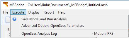
24 d) e) f) Fig. 3. Menu and submenu bars: a) menu bar; b) menu File; c) menu Execute; d) menu Display; e) menu Report; and f) menu Help 6

25 2.2.1 Menu Bar The menu bar, shown in Fig. 3, offers rapid access to most MSBridge main features. The main features in MSBridge are organized into the following menus: File: Controls reading, writing and printing of model definition parameters, exporting the mesh to other software such as SAP2000 and AutoCAD, GiD ( and Matlab, and exiting MSBridge. Please note that exporting to SAP2000.s2k file will work only if all of the following conditions are met (for now): 1) The column is linearly elastic 2) The abutment model is Elastic or Roller 3) The foundation must be Rigid-Base or Foundation Matrix 4) There is no Deck Hinge, no Isolation Bearing or no Steel Jacket, and 5) Analysis option is Pushover (monotonic) or Mode Shape Analysis Execute: Controls running analyses and OpenSees analysis parameters. Display: Controls displaying of the analysis results. Report: Controls creating the analysis report in Microsoft Word format Help: Visit the MSBridge website and display the copyright/acknowledgment message (Fig. 4). Note that Fig. 3a shows a Lock Model button which is a toggle button that prevents from overwriting analysis results after the analysis is done. If the model is in Locked Mode, all OK buttons (and Apply buttons) are disabled and users cannot make changes to the current model. To unlock the model, users need to click the Lock Model button. If the model is in Unlocked Mode, analysis results (if any) will be overwritten if analysis is launched. 7

26 Fig. 4. MSBridge copyright and acknowledgment window Model Input Region The model input region controls definitions of the model and analysis options, which are organized into three regions (Fig. 2): Step 1: Define Model & Check Responses: Controls definitions of bridge parameters including material properties. Meshing parameters are also defined in this step. Step 2:Select Analysis Option: Controls analysis types (pushover analysis, mode shape analysis or ground shaking). Equivalent Static Analysis (ESA) option is also available. Step 3: Run FE Analysis: Controls execution of the finite element analysis and display the analysis progress bar Finite Element Mesh Region The Finite Element (FE) mesh region (Fig. 2) displays the generated mesh. In this window, the mesh can be manipulated by clicking buttons shown in Fig. 5. The FE mesh shown in MSBridge is automatically generated. The user can also click the button at the top-right corner (shown in Fig. 5) to re-draw the FE mesh (based on the input data entered). 8

27 Fig. 5. Available actions in the FE Mesh window 9

28 3 BRIDGE MODEL In MSBridge, the bridge deck, columns and bentcaps are modeled using beam-column elements.the foundation is fixed-based type by default (Fig. 2). Other available foundation types including soil springs and foundation matrix are modeled using zerolength elements. To define a bridge model, click corresponding buttons Fig. 6.To include a deck hinge, isolation bearing or use a non-zero skew angle for any bent or abutment, click Advanced. To change the numbers of beam-column element used for the deck, bentcaps and columns, click Mesh. Fig. 7 shows a bridge model with soil springs and deck hinges included. Fig. 6. Model builder buttons 10

29 Fig. 7. MSBridge main window (bridge model with soil springs and deck hinges included) 3.1 Spans To change the number of spans, click Spans in the main window (Fig. 6 andfig. 8). Number of Spans: The total number of spans for a multi-span bridge. The minimum is 2 and the default value is 4. The maximum allowable number of spans is 100. MSBridge supports models for both Straight Bridge and Curved Bridge options Straight Bridge If the bridge has equal span lengths, click Equal Span Length and specify the span length (Fig. 8). The default is 60 feet. If the bridge has varied span lengths, click Varied Span Length and then Modify Span Lengths to specify span lengths (Fig. 9).Fig. 10 shows a sample straight bridge model with varied span lengths. 11

30 Fig. 8. Spans Fig. 9. Varied span lengths Fig. 10. Straight bridge with different span lengths 12

31 3.1.2 Curved Bridge To define a curved bridge, please checkhorizontal Alignment and/or Vertical Alignment infig Horizontal Curved Bridge To define a horizontally curved bridge, check Horizontal AlignmentinFig. 8. Fig. 11 shows the window to define the horizontal curves. Begin Curve Length refers to the starting location of the horizontal curve (see Fig. 12a). Curve Radius refers to the radius of the horizontal curve,curve Length refers to the arc length of the horizontal curve. And the directions (Left or Right) refers to the arc rotation direction relative to the starting location (Right: clockwise rotation in XY plan view; Left: counter-clockwise in XY plan view). Click Insert Curve to add a horizontal curve and click Delete Curve to remove the chosen curve. Fig. 14 shows examples of horizontal alignment Vertical Curved Bridge To define a vertically curved bridge, check Vertical AlignmentinFig. 8.Fig. 13shows the window to define the vertical curves. Begin Curve Length refers to the starting location of the beginning slope of the vertical curve (see Fig. 12b). Curve Length refers to the length of the vertical curve. End CurveSlope refers to the slope of the end slope. Note that the slope value can be negative, zero or positive. Similarly, Click Insert Curve to add a horizontal curve and click Delete Curve to remove the chosen curve. Fig. 15 shows examples of horizontal and vertical alignment. Note that the horizontal curve/alignment employs the circular arc while the vertical curve/alignment employs the parabolic equation. Any two (horizontal or vertical) curves cannot be overlapped and any newly added curves must be located outside all previous curves. For the detailed technical information on the horizontal & vertical alignments, please refer to the CalTrans Course Workbook for Land Surveyors (2011). 13

32 Fig. 11. Horizontal alignment a) Fig. 12. Horizontal and vertical alignments: a) horizontal alignment (plan view); b) vertical alignment (side view) b) 14

33 Fig. 13. Vertical alignment 15

34 a) b) c) Fig. 14. Examples of horizontal curved bridges (horizontal alignment): a) single radius horizontal curve; b) multi-radius horizontal curve; c) horizontal curve connecting to straight parts). 16

35 a) b) c) d) Fig. 15. Examples of vertically curved bridges (vertical alignment): a) single slope; b) begin and end slopes; c) multiple slopes; d) mixing slope and zero-slope. 17

36 3.2 Deck Sections To change Deck properties, click Deck in Fig. 6. Fig. 16 shows the window to modify the deck material and section properties. MSBridge uses an elastic material model for the bridge deck elements. Fig. 16 shows the default values for the deck material properties includingyoungs Modulus, Shear Modulus, and Unit Weight. Fig. 16. Material properties of the bridge deck Fig. 16 also shows the deck Section properties. Section properties can be input directly in Fig. 16, if available. If this information is not available MSBridge will generate properties based on general box girder section dimensions. Click Recalculate Section from Box GirderinFig. 16to define the new box girder shape (Fig. 17). The default values of geometrical properties are of typical for a four-cell reinforced concrete box girder deck configuration. Weight per Unit Length is equal to the Area of Cross Section times the Unit Weight defined in Fig. 16. Click OK in Fig. 17 if the user would like to use the defined cross section. Corresponding entries in Fig. 16will be updated. IMPORTANT NOTE: If using self-defined section properties the Box Width in Fig. 17 will be used as the deck width of the bridge. To use a different deck width, the user needs to modify Box Width in Fig

37 Fig. 17. Box girder shape employed for the bridge deck 19

38 3.3 Bentcap Sections To change bent cap properties, click Bentcap in Fig. 6. Fig. 18 shows the window to modify the bentcap material and section properties. MSBridge uses an elastic material model for the bridge bentcap elements. Fig. 18 shows the default values for the bentcap material properties includingyoungs Modulus, Shear Modulus, and Unit Weight. Fig. 18 also shows the bentcap Section properties. Section properties can be input directly in Fig. 18, if available. If this information is not available MSBridge will generate properties based on a rectangular section dimensions. Click Recalculate Section from Rectangular infig. 18to define the new rectangular shape (Fig. 19). Weight per Unit Length is equal to the Area of Cross Section times the Unit Weight defined in Fig. 18. Click OK in Fig. 17 if the user would like to use the defined cross section. Corresponding entries in Fig. 18will be updated. Fig. 18. Material properties of the bent cap 20

39 Fig. 19. Rectangular shape employed for the bent cap 21

40 3.4 Column Cross Sections To define the material and geometrical properties of column, click Column Properties in Fig. 44. For now, all columns will assume to have the same material and geometrical properties. Uses can choose to use the linearly elastic column or nonlinear Fiber column. By default, the nonlinear Fiber section is used (Fig. 20). Fig. 20. Column properties and available beam-column element types Cross Section Shapes The cross sections currently available in MSBridge include Circle, Octagon, Hexagon and Rectangle (Fig. 20). For the Circular, Octagonal and Hexagonal sections, the user 22

41 needs to define the Column Diameter. For Rectangular section, the user needs to define the widths in bridge longitudinal and transverse directions (Fig. 20) Cross Section Types Linearly Elastic To activate the linear column, check the checkbox Column is Linearly Elastic (Fig. 21). Elastic beam-column element (elasticbeamcolumn, McKenna et al. 2010) is used for the column in this case. Click Elastic Material Propertiesto define Youngs Modulus, Shear Modulus and Unit Weight of the column (Fig. 22). Click Section Properties to change the column section properties (by changing the cracked section factors) as shown in Fig Nonlinear Fiber Section To use nonlinear Fiber section for the column, click Nonlinear Fiber Section(Fig. 20). The window for defining the Fiber section is shown in Fig. 24. Click Material Properties buttons to define the material properties for the rebar, the core and the cover concrete (Fig. 25). Nonlinear beam-column elements with fiber section for the circular cross section (Fig. 26) are used to simulate the column in this case. The calculations of fibers for the octagonal and hexagonal cross sections are similar to that of the circular cross section except for the cover. Fig. 27 shows a slightly treatment of fiber calculations for the octagonal and hexagon cross sections. For Rectangular section, the number of bars refers to the number of reinforcing bars around the section perimeter (equal spacing). Two types of nonlinear Beam-Column Elements are available for the column: Beam With Hinges and Force-Based Beam Column (McKenna et al. 2010). By default, Forced-based beam-column elements (nonlinearbeamcolumn, McKenna et al. 2010) are used (the number of integration points = 5). The default values for the material properties of the column are shown in Tables 2-4. When the Beam With Hinges Element is used, the calculation of the plastic hinge length (Lp) for the column is based on Eq of SDC (2010): Where L is the column height, fye is the steel yield strength,dbl is the longitudinal bar size. The plastic hinge length (Lp) is the equivalent length of column over which the plastic curvature is assumed constant for estimating plastic rotation (SDC 2010). 23

42 The material options available for the steel bar include Elastic, Steel01, Steel02 and ReinforcingSteel. The material options available for the concrete include Elastic, ENT (Elastic-No Tension), Concrete01, and Concrete02. Fig. 21. Definition of linear column Fig. 22. Column Elastic material properties 24

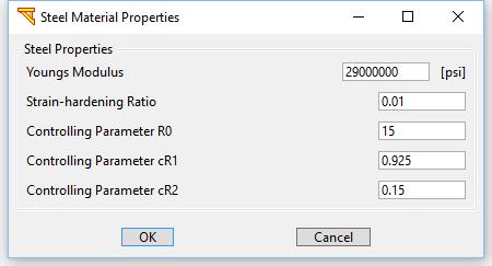
43 Fig. 23. Column Section properties By default, the Steel02 material in OpenSees (McKenna et al. 2010) is employed to simulate the steel bars and Concrete02 material is used for the concrete (core and cover). Steel02 is a uniaxial Giuffré-Menegotto-Pinto material that allows for isotropic strain hardening. Concrete02 is a uniaxial material with linear tension softening. The Concrete02 material parameters were obtained from the Mander (1988) constitutive relationships for confined and unconfined concrete. More details on the derivation of the default values and the OpenSees uniaxialmaterial definitions used for each material are shown in Appendix A. Fig. 28, Fig. 29, and Fig. 30 show the stress-strain curves for the steel, core, and cover concrete materials, respectively (The stress-strain curve is only calculated up to 6% of strain). These plots can be obtained for updated material properties directly from the interface by clicking on the corresponding View Stress-Strain buttons in the Column Material Properties window (Fig. 24). The moment-curvature response for the column is shown in Fig. 31 (generated with consideration of the overall deck weight 2680 kip applied at the column top). For comparison, XSECTION (CalTrans, 1999) result is also available (Fig. 31). Fig. 24. Nonlinear Fiber Section window 25

44 a) b) 26

45 c) d) Fig. 25. Column nonlinear material properties: a) Steel02 material; b) ReinforcingSteel material; c) Concrete02 material for the core concrete; d) Concrete02 material for the cover material 27

46 Fig. 26. Column fiber section (based on PEER best modeling practices report, Berry and Eberhard, 2007): a) Circle; b) Octagon; c) Hexagon a) b) Fig. 27. OpenSees quadrilateral patch employed for calculating the cover concrete fibers for: a) Octagon; and b) Hexagon cross section Table 1. Default values for column reinforced concrete (RC) section properties Parameter Value Longitudinal bar size (US #) 10 Longitudinal steel % 2 Transverse bar size (US #) 7 Transverse steel % 1.6 Steel unit weight (pcf) 490 Steel yield strength (psi) Concrete unit weight (pcf) 145 Concrete unconfined strength (psi)

47 Table 2. Default values for Steel02 material properties Parameter Value Typical range Steel yield strength (psi) ,000-68,000 Young s modulus (psi) 29,000,000 - Strain-hardening ratio* Controlling parameter R0** Controlling parameter cr1** Controlling parameter cr2** *The strain-hardening ratio is the ratio between the post-yield stiffness and the initial elastic stiffness. **The constants R0, cr1 and cr2 are parameters to control the transition from elastic to plastic branches. Table 3. Default values for Concrete02 material properties Parameter Core Cover Elastic modulus (psi) 3,644,147 3,644,147 Compressive strength (psi) -6, Strain at maximum strength Crushing strength (psi) -6,538 0 Strain at crushing strength Ratio between unloading slope Tensile strength (psi) Tensile softening stiffness (psi) 255, ,000 29

48 a) b) c) Fig. 28. Stress-strain curve for a steel material (default values employed): a) Steel01 (with a strain limit); b) Steel02 (with a strain limit); and c) ReinforcingSteel (with a strain limit) 30

49 a) b) c) Fig. 29. Stress-strain curve of the core concrete material (default values employed): a) Elastic-No Tension; b) Concrete01; and c) Concrete02 31

50 a) b) Fig. 30. Stress-strain curve of the cover concrete material (default values employed): a) Concrete01; and b) Concrete02 32

51 Fig. 31. Moment-curvature response for the column (with default steel and concrete parameters, and the deck weight 2500 kip applied at the column top User-defined Moment Curvature Fig. 32. User-defined moment curvature 33

52 User-defined Tcl Script for Nonlinear Fiber Section Fig. 33. User-defined Tcl script for nonlinear fiber section 34

53 3.5 Foundation Rigid Base There are three types of foundations available (Fig. 34): Rigid Base, Soil Springs and Foundation Matrix. If Rigid Base is chosen, all column bases will be fixed (in 3 translational and 3 rotational directions). In that case, the fixity nodes of the abutment models are also fixed. Fig. 34. Foundation types available in MSBridge Soil Springs To define soil springs, choose Soil Springs(Fig. 34) and then click ModifySoil Springs to define soil spring data or clickmodify Shaft Foundation to define pile shaft data (Fig. 34). It is possible to include a shaft foundation at particular bents or abutments, simply check the box to turn off/on shaft foundation for each bent/abutment. Parameters defining the pile foundation include (Fig. 35): Pile Diameter: the diameter of the pile shaft (the cross section is assumed to be circular), which is 48 in by default. Young s Modulus: Young s Modulus of the pile shaft. The foundation piles are assumed to remain linear. Pile Group Layout (see Fig. 35). This option allows defining the numbers of pile as well as the spacing (in the bridge longitudinal and transverse directions). For now, this option is only available for both abutments. For a bent, one single pile is assumed. 35

54 Fig. 35. Shaft foundation for abutments and bents When implementing the soil springs for an abutment section consider Fig. 36 as a representation of the model. The abutment nodes are the same nodes that will be referred to in the abutment model section. These nodes are described as the fixities in each of the SDC models figures. Fig. 36. Pile foundation model for abutments 36

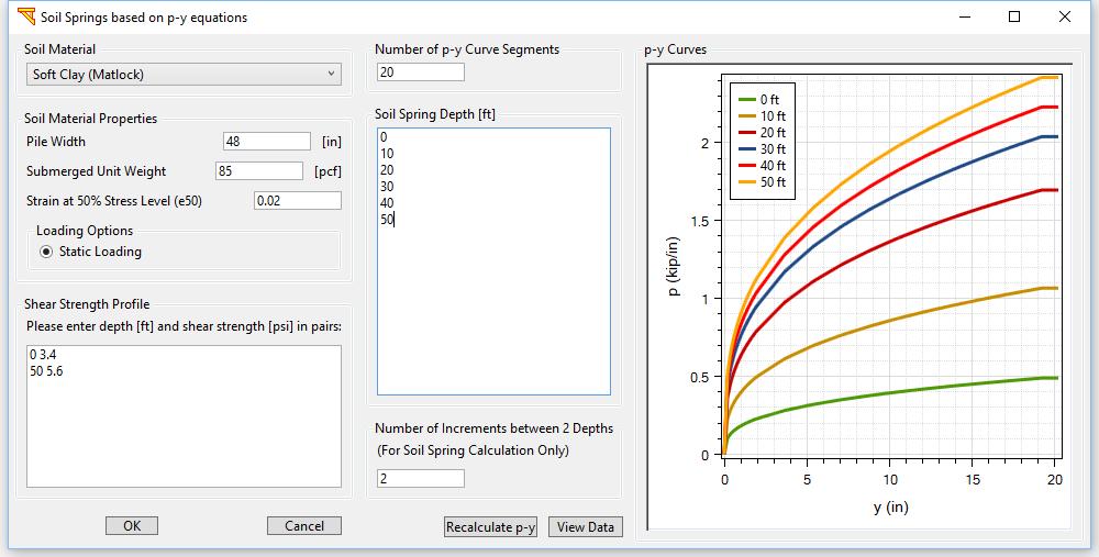
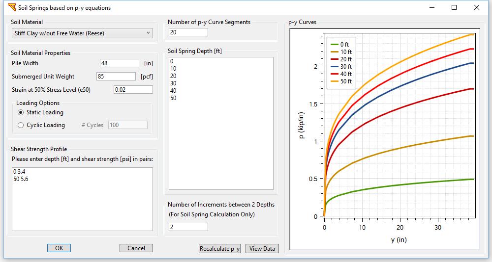
55 Parameters defining soil springs are shown in Fig. 37. Two identical horizontal soil springs (one for the bridge longitudinal direction and the other one for the transverse direction) will be applied at each depth. Button Insert Depth inserts a depth after the current depth being highlighted. Button Delete Depth removes the current depth being highlighted (as well as the associated soil spring data). To calculate the soil spring data based on p-y equations, click Select from p-y Curves (Fig. 37). For now, three types of soil p-y curves are available: Soft Clay (Matlock), Stiff Clay with no Free Water (Reese), and Sand (Reese).Fig. 38 show the calculated p-y curves for the above mentioned soil materials, respectively. The methods to calculate these p-y curves are based on the procedures described in the reference by Reese and van Impe (2001). To use the soil spring data calculated based on p-y curves, click OK and then click Yes. The soil spring data chosen will replace the existing any soil spring data (Fig. 39). A sample bridge model with soil springs included is shown in Fig. 40. Fig. 37. Soil springs 37

56 a) b) 38

57 c) d) Fig. 38. Soil spring calculations based on p-y equations: a) Soft Clay (Matlock); b) Stiff Clay without Free Water (Reese); c) Sand (Reese); d) Liquefied Sand (Rollins) 39

58 Fig. 39. Soil spring definition window after using the soil spring data calculated based on p-y equations Fig. 40. Sample FE mesh of a bridge model with soil springs included Foundation Matrix The third foundation type available is Foundation Matrix (Fig. 34, Li and Conte 2013). In this method, the foundation (only for bent columns) is represented by the coupled 40

59 foundation stiffness matrix (Lam and Martin 1986). Specifically, the stiffness of a single pile is represented by a 6 x 6 matrix representing stiffness associated with all six degrees of freedom at the pile head. The local coordination system employed for the foundation matrix is parallel to the global coordination system (Fig. 41). To define foundation matrix, select Foundation Matrix and then click Modify Foundation Matrix(Fig. 34). Fig. 42 shows the window defining the foundation matrix for the column base of each bent. To apply the matrix defined for any bent for the remaining bents, select that bent in the Bent No box and then check Use this Matrix for All Other Bents. Fig. 41. Local coordination system for the foundation matrix 41

60 Fig. 42. Foundation matrix for each bent 42

61 3.6 Abutment Fig. 43. Definition of an abutment model 43

62 3.7 Bridge Model To modify column properties, click Columns in Fig. 6.Fig. 44 shows the window to define columns. The current version assumes that all bents have the same number of columns, and the same Column Spacing. If Number of Column for Each Bent is 1, Column Spacing will be ignored (Fig. 44). Fig. 44. Columns 44

63 3.7.1 Column Heights To define column heights, click ModifyColumn Heights in Fig. 44. A window for defining column heights will appear (Fig. 45) Column Connection Fig. 45. Column heights In a multi-column case (the number of columns per bent is equal to 2 or more), the user can specify the boundary connection conditions of the columns. Click Column Connection (in Fig. 44) to select the boundary condition for the columns and bent cap connection. Three options are available (Fig. 46): i) fixed at top / pinned at base; ii) pinned at top / fixed base; and iii) fixed at both top and base. Note: In a single column case (the number of columns per bent is equal to 1), both column top and base are assumed fixed. Fig. 46. Column boundary conditions 45

64 a) b) Fig. 47. Bridge configuration: a) general options; b) column layout Steel Jackets To define steel jackets, click DefineSteel Jacketsin Fig. 50 and a window for defining steel jacket properties will appear (Fig. 48). For now, the steel jacket option is only available to the circular column. To activate/define steel jacket for all columns for a bent, please nonzero values for the corresponding row (Fig. 48). In the case of partial length of steel jacket (Fig. 49), please specify enough number of elements for the column (since the equal size of elements is used for the columns within a bent, for now). The steel properties used in the steel jacket implementation are the same as user defined properties for the steel reinforcement of the column shown in Fig

65 Fig. 48. Definition of steel jackets Fig. 49. Sketch of steel jacket 47

66 3.8 Advanced Options The advanced options in MSBridge include Deck Hinges, Isolation Bearings and Skew Angles. Click Advanced in Fig. 6 to include any of these options as shown infig. 50into the bridge model Deck Hinges Fig. 50. Advanced options To define deck hinges, click DefineDeck Hingesin Fig. 50 and a window for defining deck hinge properties will appear (Fig. 51). A sample bridge model including 2 deck hinges is shown in Fig

67 Fig. 53 shows the general scheme of a Deck Hinge, which consists of 2 compression connectors (located at both deck edges) and cables. To activate/define a deck hinge, check the checkbox immediately prior to the Hinge # (e.g., Hinge 2). Distance to Bent: The distance to the nearest (left) bent. Foot and meter are used for English and SI units, respectively Spacing: The space between transverse left and right deck connectors. This space should usually approximately equal to the Deck Width. Skew Angle: The skew angle of the deck hinge. A zero skew angle means the deck hinge is perpendicular to the bridge deck direction # of Cables: The total number of cables of the deck hinge Cable Spacing: The spacing between cables. Symmetric layout of cables is assumed. Foot and meter are used for English and SI units, respectively As shown infig. 53, zerolength elements are used for cables and compression connectors. The bearing pads are included in the cables. For each zerolength element, both nodes are interacted in the longitudinal direction (denoted as direction 1 in Fig. 53) but tied in the vertical direction 3 (not shown infig. 53) as well as the transverse direction (denoted as direction 2 in Fig. 53). The above conditions would force both sides of deck segments to move in the same plane. Note that the local coordinate system may or may not coincide with the global coordinate system X-Y-Z (Fig. 1). In the longitudinal direction and as the load is applied at the right side of the hinge; only the bearings will resist the movement since the cables are loose, but once the cables start to be stretched the cables stiffness will add resistance to the movement. In addition, the connectors will be out of the picture since the gap is not closing while the load is tension. On the other hand, if the load is applied to the left side of the hinge; the gap will be closing and only the bearing will resist the movement until the gap is closed, then the connectors 49

68 and based on the their stiffnesses will make sure that the deck will move as one object. The cables are not playing any role in this process. In the transverse direction does not matter at which direction the load will be applied, the hinge will act the same. Both nodes are tied and both sides of the deck segments will move in the same plane; even if the bearing stiffness is very low. However, as the two segments are moving in the transverse direction, they will rotate and this rotation will make the nearest end in compression and the other end in tension. Therefore, the bearings and the connectors if the gap is closed - will work longitudinally in the compression end, and the bearings and cables if they are stretched will act longitudinally in the tension end. The default values of properties for the compression connectors, cables, bearing pads are also shown in Fig

69 a) b) Fig. 51. Definition of deck hinges 51

70 Fig. 52. FE mesh of a 4-span model with 2 deck hinges included Fig. 53. OpenSees zerolength elements for deck hinges (plan view) Isolation Bearings To define isolation bearings, click DefineIsolation Bearingsin Fig. 50 and a window for defining isolation bearing properties will appear (Fig. 54). A sample bridge model including 2 isolation bearings on each bent cap is displayed in Fig. 55. To activate/define isolation bearings on a bent cap, check the checkbox immediately prior to the Bent # (e.g., Bent 2). # Bearings: The total number of isolation bearings implemented at the bent cap. Spacing: The spacing between isolation bearings. A symmetric layout of bearings is assumed. The default values of material properties for the isolation bearings are also shown in Fig. 54. As shown in Fig. 56, zerolength elements are used for the isolation bearings (Li and 52

71 Conte, 2013). For each zerolength element, the 2 nodes are interacted in both horizontal directions (denoted as directions 1 (not shown) and 2 infig. 56) but tied in the vertical direction 3 (Fig. 56). Note that the local coordinate system may or may not coincide with the global coordinate system X-Y-Z (Fig. 1). Fig. 54. Definition of isolation bearings Fig. 55. FE mesh of a 4-span bridge model with 2 isolation bearings included on each bent cap 53

72 Fig. 56. OpenSees zerolength elements for isolation bearings (side view of bent cap cutplan) Skew Angles The user can choose to use a single (global) skew angle or individual skew angles for abutments and bents. By default, a zero Global Skew Angle is assumed (Fig. 57). To define individual skew angles, check the checkbox Use Individual Skew Angles. To define individual skew angles, click Bents and Abutmentsin Fig. 57a. A window for defining skew angle properties will appear (Fig. 57b). Fig. 57. Definition of skew angles 54

73 Fig. 58. Definition of pilecap mass Fig. 59. Definition of steel jackets 55

74 3.9 Mesh Parameters To change the number of beam-column elements for the bridge model, click Mesh infig. 6.Fig. 60 displays the Mesh Parameters window showing the default values. The number of beam-column elements for a deck segment (a span) must be least 2. And for the bent cap segment between columns, the number of elements must be even. Fig. 60. Mesh parameters 56

75 4 ABUTMENT MODELS Abutment behavior, soil-structure interaction, and embankment flexibility have been found by post-earthquake reconnaissance reports to significantly influence the response of the entire bridge system under moderate to strong intensity ground motions. Specifically, for Ordinary Standard bridge structures in California with short spans and relatively high superstructure stiffness, the embankment mobilization and the inelastic behavior of the soil material under high shear deformation levels dominate the response of the bridge and the intermediate column bents (Kotsoglu and Pantazopoulou, 2006, and Shamsabadi et al. 2007, 2010). Seven abutment models have been implemented in MSBridge. The abutment models are defined as Elastic, Roller, SDC 2004, SDC 2010 Sand, SDC 2010 Clay, EPP-Gap and HFD abutment models. To define an abutment model, click Abutments in Fig. 6.A window for defining an abutment model is shown in Fig Elastic Abutment Model The Elastic Abutment Model consists of a series of 6 elastic springs (3 translational and 3 rotational) at each node at the end of the bridge (Fig. 62). To choose the Elastic Abutment Model, select Elastic for the Model Type in Fig. 61 (Fig. 63).The main window to define the Elastic Abutment Model is shown in Fig. 64. By default, no additional rotational springs are specified, but can be added by the user. As shown infig. 62 and Fig. 64, MSBridge allows the user to define multiple distributed springs (equal spacing within deck width). The values specified in Fig. 64 are the overall stiffness for each direction (translational or rotational). For the longitudinal direction (translational and rotational), each of the distributed (Elastic) springs carries its tributary amount. e.g., Fig. 62 shows a case of 4 distributed springs. Each of the both end springs carries one-sixth of the load and each of the middle springs carries one-third (Fig. 62a). The vertical components (translational and rotational) are similar to the longitudinal ones. i.e., each of the distributed springs carries its tributary amount in the vertical direction. However, the transverse component is different: only the both end-springs carry the load. In other words, each of the end springs carries half of the load along the transverse direction (translational and rotational). By default, the number of distributed springs is 2. In this case, these 2 springs are located at the both ends of the Rigid element (the length of which is equal to deck width) shown in Fig. 62. However, due to the coupling of the longitudinal, and vertical translational springs, the option of using a single node at each abutment is possible, this gives the user full control over the true rotational stiffness apart from the translational stiffness. 57

76 Fig. 61. Definition of an abutment model The abutment will be rotated counter-clockwise if the skew angle is positive (rotated clockwise if negative). Fig. 65 shows the direction of longitudinal springs in a curved bridge with a non-zero skew angle. Fig. 66 shows a bridge model with 5 distributed abutment springs and a non-zero skew angle. 58

77 a) b) c) Fig. 62. General scheme of the Elastic Abutment Model: a) longitudinal component; b) transverse component; c) vertical component 59

78 Fig. 63. Definition of the Elastic Abutment Model Fig. 64. Parameters of the Elastic Abutment Model 60

79 a) b) Fig. 65. Longitudinal components of the Elastic Abutment Model in a curved bridge: a) left abutment; b) right abutment 61

80 a) b) Fig. 66. Bridge model with multiple distributed springs and a positive skew angle: a) straight bridge; b) curved bridge 4.2 Roller Abutment Model The Roller Abutment Model (Fig. 67) consists of rollers in the transverse and longitudinal directions, and a simple boundary condition module that applies single-point constraints against displacement in the vertical direction (i.e., bridge and abutment are rigidly connected in the vertical direction). These vertical restraints also provide a boundary that prevents rotation of the deck about its axis (torsion). This model can be used to provide a lower-bound estimate of the longitudinal and transverse resistance of the bridge that may be displayed through a pushover analysis. To choose the Roller Abutment Model, select Roller for the Model Type in Fig. 61 (and Fig. 68). 62

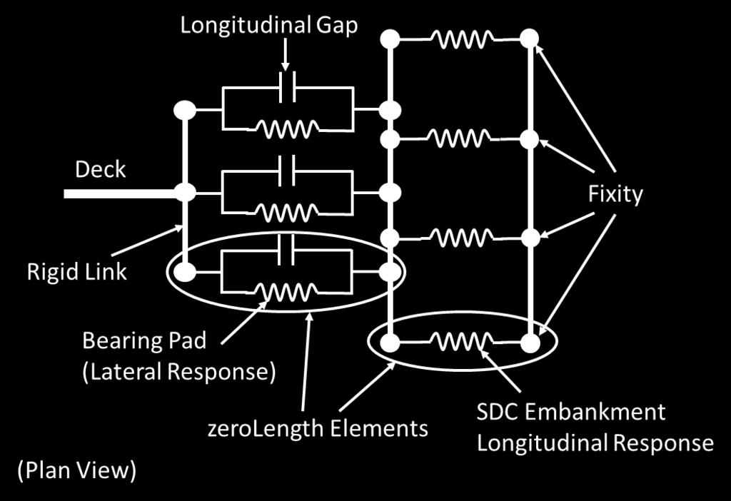
81 Fig. 67. General scheme of the Roller Abutment Model Fig. 68. Selection of the Roller Abutment Model 4.3 SDC 2004 Abutment Model SDC 2004 Abutment Model was developed based on the Spring Abutment Model by Mackie and Stojadinovic (2006). This model includes sophisticated longitudinal, transverse, and vertical nonlinear abutment response. Detailed responses of the abutment model in the longitudinal, transverse, and vertical directions are described below Longitudinal Response The longitudinal response is based on the system response of the elastomeric bearing pads, gap, abutment back wall, abutment piles, and soil backfill material. Prior to impact or gap closure, the superstructure forces are transmitted through the elastomeric bearing pads to the stem wall, and subsequently to the piles and backfill, in a series system. After gap closure, the superstructure bears directly on the abutment back wall and mobilizes the full passive backfill pressure. The detailed scheme of the longitudinal response is shown in Fig. 69a. The typical response of a bearing pad is shown in Fig. 69b. And the typical overall behavior is illustrated in Fig. 69c. The yield displacement of the bearings is assumed to be at 150% of the shear strain. The longitudinal backfill, back wall, and pile system response are accounted for by a series of zero-length elements between rigid element 2 and the fixity (Fig. 69a). The abutment initial stiffness (Kabt) and ultimate 63

82 passive pressure (Pabt) are obtained from equations 7.43 and 7.44 of SDC Fig. 70 shows the directions of zerolength elements for a curved bridge with a skew angle. Each bearing pad has a default height (h) of m (2 in) which can be modified by user and a side length (square) of m (20 in). The properties of a bearing pad are listed in Table 4. The abutment is assumed to have a nominal mass proportional to the superstructure dead load at the abutment, including a contribution from structural concrete as well as the participating soil mass. An average of the embankment lengths obtained from Zhang and Makris (2002) and Werner (1994) is included in the calculation of the participating mass due to the embankment of the abutment. The user can modify the lumped mass through the soil mass. For design purposes, this lumped mass can be ignored and set to be zero. Table 4. Geometric and Material Properties of a Bearing Pad Shear Modulus G kpa (0.15 ksi) Young s Modulus E kpa (5 ksi) Yield Displacement 150% shear strain GA Lateral Stiffness h (where A is the cross-section area and h is the height) Longitudinal gap 4 in hardening ratio 1% Vertical Stiffness Vertical Tearing Stress Longitudinal gap EA h kpa (2.25 ksi) 2 in 64

83 a) b) 65

84 c) Fig. 69. Longitudinal response of the SDC 2004 Abutment Model: a) general scheme; b) longitudinal response of a bearing pad; c) total longitudinal response 66

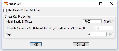
85 Fig. 70. Longitudinal response of the SDC 2004 Abutment Model for a curved bridge with a (positive) skew angle Transverse Response The transverse response is based on the system response of the elastomeric bearing pads, exterior concrete shear keys, abutment piles, wing walls, and backfill material. The bearing pad model discussed above is used with uncoupled behavior with respect to the longitudinal direction. The constitutive model of the exterior shear keys is derived from experimental tests (Megally et al., 2003). Properties (yield and ultimate stresses) of shear keys depend on ultimate capacity of the bridge which is defined as 30 percent of dead load at abutment. The detailed scheme of the transverse response is shown in Fig. 71a. The typical response of a bearing pad and a shear key is shown in Fig. 71b. And the typical overall behavior of the transverse response is illustrated in Fig. 71c. The superstructure forces are transmitted through the parallel system of bearing pads and shear keys (T1) to the embankment (T2) in series. The ultimate shear key strength is assumed to be 30% of the superstructure dead load, according to equation 7.47 of SDC A hysteretic material with trilinear response backbone curve is used with two hardening and one softening stiffness values. The initial stiffness is a series-system stiffness of the shear and flexural response of a concrete cantilever with shear key dimensions (16849 ksi). The hardening and softening branches are assumed to have magnitudes of 2.5% of the initial stiffness. The transverse stiffness and strength of the backfill, wing wall and pile system is calculated using a modification of the SDC procedure for the longitudinal direction. 67

86 Wingwall effectiveness (CL) and participation coefficients (CW) of 2/3 and 4/3 are used, according to Maroney and Chai (1994). The abutment stiffness (Kabt) and back wall strength (Pbw) obtained for the longitudinal direction from Section 7.8 of SDC 2004 are modified using the above coefficients. The wing wall length can be assumed 1/2 1/3 of the back wall length. The bearing pads and shear keys are assumed to act in parallel. Combined bearing pad- shear key system acts in series with the transverse abutment stiffness and strength. a) b) 68

87 c) Fig. 71. Transverse response of the SDC 2004 Abutment Model: a) general scheme; b) response of a bearing pad and shear keys (curve with a higher peak value is the shear key response); c) total transverse response Vertical Response The vertical response of the abutment model includes the vertical stiffness of the bearing pads in series with the vertical stiffness of the trapezoidal. The detailed scheme of the vertical response is shown in Fig. 72a. The typical vertical response of a bearing pad is shown in Fig. 72b. And the typical overall behavior of the vertical response is illustrated in Fig. 72c. A vertical gap (2-inch by default, which can be modified by the user) is employed for the vertical property of the bearing pads. The embankment stiffness per unit length of embankment was obtained from Zhang and Makris (2000) and modified using the critical length to obtain a lumped stiffness. In the vertical direction, an elastic spring is defined at each end of the rigid link, with a stiffness corresponding to the vertical stiffness of the embankment soil mass. The embankment is assumed to have a trapezoidal shape and based on the effective length formulas from Zhang and Makris (2002), the vertical stiffness ( K v, unit: 1/m) can be calculated from (Zhang and Makris, 2002): 69

88 Esld w Kv = Lc ln z0 + H (3) z 0 z0 Where H is the embankment height, dw is the deck width, z = 0.5d S, S 0 w is the 2 embankment slope (parameter in window, see Fig. 20), E sl = 2. 8G, G = V s, and V s are the mass density and the shear wave velocity of the embankment soil, respectively. 70

89 a) b) c) Fig. 72. Vertical response of the SDC 2004 Abutment Model: a) general scheme; b) vertical response of a bearing pad; c) total vertical response 71

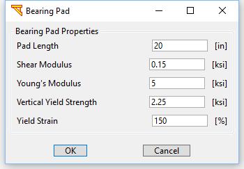
90 4.3.4 Definition of the SDC 2004 Abutment Model To define a SDC 2004 Abutment Model, please follow the steps shown in Fig. 73. To define a SDC 2004 Abutment Model, select SDC 2004 for the abutment model type in Fig. 61. The resulting window is shown in Fig. 73a. a) 72

91 b) c) 73

92 d) e) Fig. 73. Definition of the SDC 2004 Abutment Model: a) main parameters; b) bearing pad properties; c) shear key properties; d) SDC abutment properties; e) embankment properties 74

93 4.4 SDC 2010 Sand Abutment Model This model is similar to the SDC 2004 abutment model, but employs the parameters of the most recent SDC 2010 for a sand backfill Embankment (Fig. 74). To define a SDC 2010 Sand Abutment Model, select SDC 2010 Sand for the abutment model type in Fig. 61.Table 5 shows the initial stiffness and the maximum passive pressure employed for the SDC 2010 Sand Abutment Model, compared to other similar abutment models including SDC 2004, SDC 2010 Clay, EPP-Gap and HFD Models). Fig. 74. Backfill horizontal properties for the SDC 2010 Sand Abutment Model Table 5. SDC Abutment Properties Abutment Model Initial Stiffness Maximum Passive Pressure (kip/in/ft) (ksf) SDC SDC 2010 Sand 50 5 SDC 2010 Clay 25 5 EPP-Gap User-defined User-defined HFD Model *50 (sand); 25 (clay) 5.5 *Denotes average soil stiffness K50. 75

94 4.5 SDC 2010 Clay Abutment Model This model is similar to the SDC 2004 abutment model, but employs the parameters of the most recent SDC 2010 for a Clay backfill Embankment (Fig. 75). To define a SDC 2010 Clay Abutment Model, select SDC 2010 Clay for the abutment model type in Fig. 73a. Table 5 shows the initial stiffness and the maximum passive pressure employed for the SDC 2010 Clay Abutment Model, compared to other similar abutment models. Fig. 75. Backfill horizontal properties of the SDC 2010 Clay Abutment Model 4.6 ElasticPP-Gap Model This model is similar to the SDC 2004 Abutment Model, but employs user defined parameters for the stiffness and maximum resistance (Fig. 76). To define anepp-gap Abutment Model, select EPP-Gap for the abutment model type in Fig

95 Fig. 76. Backfill horizontal properties of the EPP-Gap Abutment Model 4.7 HFD Model As suggested by Shamsabadi et al. (2007, 2010), a Hyperbolic Force-Displacement (HFD) relationship is employed to represent abutment resistance to bridge displacement in the longitudinal direction (Fig. 77). F(y) = F ult (2K 50 y max F ult )y F ult y max + 2(K 50 y max F ult )y Where F is the resisting force, y is the longitudinal displacement, Fult is the ultimate passive resistance and K50 is the secant stiffness at Fult/2. 77

96 F(y) = (2K 50 F ult y max ) y ( K 50 F ult 1 y max ) y In this HFD model, resistance appears after a user-specified gap is traversed, and the bridge thereafter gradually mobilizes the abutment s passive earth pressure strength. Herein, this strength is specified according to Shamsabadi et al. (2007, 2010) at 5.5 ksf (for a nominal 5.5 ft bridge deck height), with full resistance occurring at a passive lateral displacement of 3.6 in (the sand structural backfill scenario). Similarly, abutment resistance to the transverse bridge displacement is derived from the longitudinal hyperbolic force-displacement relationship according to the procedure outlined in Aviram et al. (2008). To define a HFD abutment model, select HFD Model for the abutment model type in Fig. 73. Click Advanced in Embankment Lateral Stiffness box (Fig. 73) to define the backfill horizontal properties (Fig. 77c). Parameters of the backfill soil are defined based on soil types (sand, clay, or User-defined) and the overall abutment stiffness/ or maximum passive pressure resist are calculated using the SDC equations. a) 78

97 b) c) Fig. 77. Definition of the HFD Abutment Model: a) HFD abutment model; and b) HFD parameters for abutment backfills suggested by Shamsabadi et al. (2007); and c) backfill properties of the HFD Model 79

98 5 COLUMN RESPONSES & BRIDGE RESONANCE MSBridge provides features to view column lateral responses, abutment responses and bridge natural periods (Fig. 7 and Fig. 78). Fig. 78. Buttons to view column & abutment responses and bridge resonance 5.1 Bridge Natural Periods Click View Natural Periods (Fig. 78) to view the natural periods and frequencies of the bridge (Fig. 79). A mode shape analysis is conducted in this case. The user can copy and paste the values to their favorite text editor such as MS Excel (in Fig. 79, right-click and then click Select All (ctrl a) to highlight, and then right-click and then click Copy (ctrl c) to copy to the clipboard). 5.2 Column Gravity Response Click View Gravity Response (Fig. 78) to view the column internal forces and bending moments after application of own weight (Fig. 80). 5.3 Column & Abutment Longitudinal Responses Click Longitudinal Response (Fig. 78) to view the column longitudinal responses (Fig. 81) and the abutment longitudinal responses (Fig. 82). A pushover up to 5% of drift ratio in the longitudinal direction is conducted in this case. 5.4 Column & Abutment Transverse Responses Click Transverse Response (Fig. 78) to view the column transverse responses (Fig. 83) and the abutment transverse responses (Fig. 84). A pushover up to 4% of drift ratio in the transverse direction is conducted in this case. 80

99 Fig. 79. Natural periods and frequencies of bridge Fig. 80. Column internal forces and bending moments after application of own weight 81

100 Fig. 81. Column longitudinal responses Fig. 82. Abutment longitudinal responses 82

101 Fig. 83. Column transverse responses Fig. 84. Abutment transverse responses 83

102 6 PUSHOVER & EIGENVALUE ANALYSES 6.1 Pushover Analysis To conduct a pushover analysis, a load pattern must be defined. As shown in Fig. 85, first, choose Pushover in the Analysis Options, and then click Change Pattern. The load pattern window is shown in Fig Input Parameters Monotonic Pushover Fig. 85. Pushover analysis option The pushover options include Monotonic Pushover, Cyclic Pushover, andu-push (pushover by a user-defined loading pattern). Two methods of pushover are available (Fig. 86): force-based and displacement-based. If Force-Based Method is chosen, please enter the parameters of force increment (per step): Longitudinal (X) Force, Transverse (Y) Force, Vertical (Z) Force, X, Y, and Z. If Displacement-Based Method is chosen, please enter the displacement increment parameters (per step): Longitudinal Displacement, Transverse Displacement, Vertical Displacement, Rotation around X, Rotation around Y, and Rotation around Z. The pushover load/displacement linearly increases with step in a monotonic pushover mode. The pushover load/displacement is applied at the bridge deck center or the deck location at a bent. 84

103 Cyclic Pushover Fig. 86. Load pattern for monotonic pushover analysis To conduct a Cyclic Pushover, click Cyclic PushoverinFig. 86and then define Number of Steps for the First Cycle and Step Increment per Cycle (Fig. 87). Fig. 87. Load pattern for cyclic pushover analysis User-Defined Pushover (U-Push) Click U-Push and then click Define U-Push to enter your own load pattern (U-Push). In this case, the displacement or force parameters entered in Fig. 88 are used as the 85

104 maximum values. The U-Push data entered are used as the factors (of the maximum displacement or the maximum force entered) Output for Pushover Analysis Fig. 88. User-defined pushover (U-Push) Output windows for a pushover analysis include: i) Response time histories and profiles for column (and pile shaft under grade) ii) Response relationships (force-displacement as well as moment-curvature) for column (and pile shaft under grade) iii) Abutment response time histories iv) Deformed mesh, contour fill, plastic hinges, and animations. 86

105 Column Response Profiles Fig. 89. Column response profiles 87

106 Column Response Time Histories Fig. 90. Column response time histories 88

107 Column Response Relationships Fig. 91. Response relationships for column 89

108 Abutment Force-Displacement and Response Time Histories Fig. 92. Abutment response time histories 90

109 Deformed Mesh Fig. 93. Deformed mesh and contour fill 91

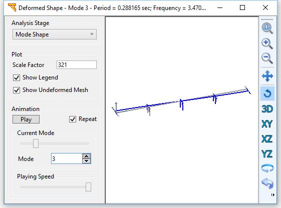
110 Fig. 94. Visualization of Plastic hinges (red dots represent plastic hinges developed) 6.2 Eigenvalue Analysis To conduct an Eigenvalue analysis, please follow the steps shown in Fig. 95 and then click Save Model & Run Analysis. Fig. 96 shows the output window for an Eigenvalue analysis, which can be accessed by clicking menu Display (Fig. 3) and then choosing Deformed Mesh. To switch between modes, move the slideror click the spin button to cycle through them. Fig. 95. Steps to perform an Eigenvalue analysis 92

111 a) 93

112 b) 94

113 c) 95

114 d) 96

115 e) Fig. 96. Sample output for an Eigenvalue analysis for the default bridge model: a) first mode; b) second mode; c) third mode; d) fourth mode; and e) fifth mode 97

116 7 GROUND SHAKING To conduct a single earthquake analysis or a multiple earthquake analyses, the Ground Shaking option under Analysis Options (Fig. 2 and Fig. 97) is used. For that purpose, the input earthquake excitation(s) must be specified. If only one earthquake record is selected out of a specified ensemble (suite) of input motions, then a conventional single earthquake analysis will be performed. 7.1 Definition/specification of input motion ensemble (suite) Available Ground Motions A set of 20 motions provided by CalTrans are available as the default input motion package. The above ground motion data sets were resampled to a sampling frequency of 50 Hz (regardless of whether initial sampling frequency was 100 or 200 Hz) due to the computational demands of running full ground-structure analyses for an ensemble of motions. Standard interpolation methods were used to resample the time domain signals (so that the signal shape is preserved). The resampled records were then baselined to remove any permanent velocity and displacement offsets. Baselining was accomplished using a third order polynomial fitted to the displacement record. In addition, four sets of input motions are also available (can be downloaded from the website: Motion Set 1: These 100 motions were obtained directly from the PEER NGA database and all files have been re-sampled to a time step of 0.02 seconds. This PBEE motion ensemble (Medina and Krawinkler 2004) obtained from the PEER NGA database ( consists of 100 3D input ground motions. Each motion is composed of 3 perpendicular acceleration time history components (2 lateral and one vertical). These motions were selected through earlier efforts (Gupta and Krawinkler, 2000; Mackie et al., 2007) to be representative of seismicity in typical regions of California. The moment magnitudes (Mw) of these motions range from (distances from 0-60 km). The engineering characteristics of each motion and of the ensemble overall may be viewed directly within MSBridge. The provided ground motions are based on earlier PEER research (Mackie and Stojadinovic 2005). Motion Set 2: These motions (160 in total) were developed by Dr. Kevin Mackie from the 80 motions of Set1 (excluding the 20 motions of Set1 in the bin NEAR), to account for site classification. Motion Set 3: These motions (80 in total) were developed by Dr. Jack Baker for PEER. Additional information about these motions is available at the website: 98

117 Motion Set 4: These motions (260 in total) include the above Set2 and Set3 as well as the additional Bin NEAR of Set1. Once an input motion data set is specified, the user interface will extract/calculate Intensity Measures (IMs) for each of these motions. In total, 11 different Intensity Measures are defined for each motion (and presented to the user in table and graphical forms), including quantities such as Peak Ground Acceleration (PGA), Peak Ground Velocity (PGV), Arias Intensity (AI), and so forth Specifications of Input Motions To conduct a ground shaking analysis, input motions must be defined Fig. 97). The window to define input motions is shown in Fig. 98. To select all motions, click Select All. To un-select all motions, click De-select All.To remove one motion, select the motion by clicking on it and then click Delete. To remove all motions, click Remove All. To add a user-defined motion, click Import and then follow the simple steps to import a new motion (Fig. 99). The resulting motion will be added to the current suites of input motion. To obtain a complete new set of input motions, use Delete All to remove all existing input motions, and then use Import to add new motions. To import a ground motion file, first save the ground acceleration time history (easy in a notepad.txt file) with each new line being the next acceleration time step. This data in this file should have the acceleration units of g. The finite element computations can be conducted for several earthquakes at a time. This is employed by specifying Number of Motions Running Simultaneously (Fig. 98). You can select as many as 8 records to be run at the same time in order to reduce the overall run time (for dual core machines or better). Click View Motion to view the intensity measures and response spectra of the input motion being highlighted (Fig. 100). SRSS stands for Square Root of the Sum of the Squares of the 2 horizontal components. Click Display Intensity Measures to view the intensity measures of the input motion being highlighted (Fig. 101). The user can copy and paste the intensity measures to their favorite text editor such as MS Excel (in Fig. 101, right-click and then click Select All (ctrl a) to highlight, and then right-click and then click Copy (ctrl c) to copy to the clipboard). Click View Histograms & Cumulative Distribution to view the histogram and cumulative distribution plots for whole input motion set (Fig. 102). The intensity measures include: PGA (Peak Ground Acceleration) PGV (Peak Ground Velocity) PGD (Peak Ground Displacement) D5-95 (Strong Motion Duration) CAV (Cumulative Absolute Velocity) 99

118 Arias Intensity SA (Spectral Acceleration; assuming 1 second period) SV (Spectral Velocity; assuming 1 second period) SD (Spectral Displacement; assuming 1 second period) PSA (Pseudo-spectral Acceleration) PSV (Pseudo-spectral Velocity) The strong motion duration (D5-95) is defined according to the time domain bounded by the 5% and 95% cumulative Arias intensity of the record. All of the spectral intensity measures are defined at an effective viscous damping of 5% unless otherwise noted. Fig. 97. Group shaking analysis 100

119 Fig. 98. Input motions window 101

120 Fig. 99. Importing a user-defined motion 102

121 Fig Time histories and response spectra of individual motion 103

122 Fig Intensity measures of individual motion 104

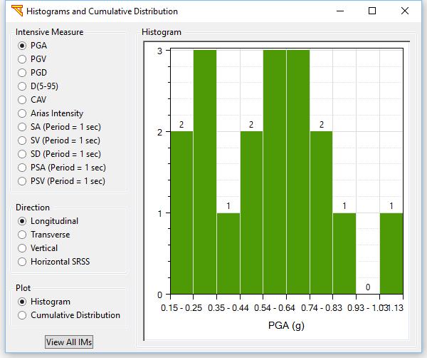
123 a) 105

124 b) Fig Histogram and cumulative distribution for the whole input motion set: a) histogram; b) cumulative distribution 7.2 Rayleigh Damping MSBridge employs Rayleigh damping, which takes the form: C = AmM + AkK wherem is the mass matrix, C is the viscous damping matrix, K is the initial stiffness matrix. Am and Ak are two user-specified constants. The damping ratio curve ( f) is calculated based on the following equation: 106

125 Am = + Ak f 4 f wheref is frequency. (1) Specification of A m and A k By Defining Damping Ratios Click Change Damping in the MSBridge main window to modify the Rayleigh damping coefficients (Fig. 103). The user can define damping coefficients (Fig. 103) by specifying two frequencies, f1 and f2 (must be between 0.1 and 50 Hz), and two damping ratios, 1 and 2 (suggested values are between 0.2% and 20%). The Rayleigh damping parameters Am and Ak are obtained by solving the follow equations simultaneously: Am 1 = + Ak f1 4 f 1 Am 2 = + Ak f 4 f 2 (2) Direct Specification of A m and A k : 2 The user can also directly define Rayleigh damping coefficients Am and Ak (Fig. 103). 7.3 Save Model and Run Analysis After defining the finite element model, click Save Model and Run Analysis. The finite element computations will start, for several earthquakes at a time (Fig. 104) as specified in the Input Motions window (Fig. 98). The user can modify the time integration scheme for the OpenSees analysis by clicking Menu Execute and then Advanced Option: OpenSees Parameters (Fig. 105). Fig. 105 shows the default parameters which are used in the analysis. 107

126 Fig Rayleigh damping 108

127 Fig Simultaneous execution of analyses for multiple motions 109

128 Fig Parameters for OpenSees analysis 110

129 8 TIME HISTORY AND ENGINEERING DEMANDING PARAMETER OUTPUT 8.1 Time History Output Quantities At the end of the FE analysis phase, time histories and bridge responses will be available of the form: i) Column Response Time Profiles ii) Column Response Time Histories iii) Column Response Relationships iv) Abutment Responses v) Deformed Mesh In addition, for multiple earthquake analysis scenarios, Intensity Measures (IMs) and response spectra for each input motion are calculated and are available for display in Table and Figure formats. Engineering Demand Parameter (EDP) Quantities and Bridge peak accelerations for all employed shaking motions are also available for display against any of the computed IMs. The post-processing capabilities can be accessed from Menu Display (Fig. 3). To display output for a different input motion, click Menu Display and then Detailed Output: Please Select Input Motion (Fig. 3d). The name of the selected input motion will also appear on the menu items (Fig. 3d). Fig Selection of an input motion 111

130 8.1.1 Deck Response Time Histories The deck response time histories can be accessed by clicking menu Display (Fig. 3) and then Deck Response Time Histories.Fig. 107 shows the window for displaying the deck longitudinal displacement time histories Column Response Profiles The column response profiles can be accessed by clicking menu Display (Fig. 3) and then Column Response Profiles. The column response window is shown in Fig The columns are labeled as: i) Column 1 of Bent 2 (see Fig. 1., the first bent starting after left abutment is denoted as Bent 2, the second as Bent 3, and so on) ii) Column 2 of Bent 2 iii) (more if any) Fig. 109 shows the bending moment in the longitudinal plane. The horizontal axis of the plot is the response name (e.g., displacement, bending moment, etc.) and the vertical axis is the elevation of the column. Zero elevation means the column base Column Response Time Histories The column response time histories can be accessed by clicking menu Display (Fig. 3) and then Column Response Time Histories.Fig. 110 shows the window for displaying the column longitudinal displacement time histories. 112

131 Fig Deck longitudinal displacement response time histories Fig Displacement profile in the longitudinal plane 113

132 Fig Bending moment profile in the longitudinal plane 114

133 Fig Response time histories and profiles for column (and pile shaft): displacement is shown at the nodes Column Response Relationships The column response relationships can be accessed by clicking menu Display (Fig. 3) and then Column Response Relationships. The Elevation box includes all elevations (starting from column top). Zero elevation refers to the colufig. 111 shows the longitudinal load-displacement curve at the column top. The load refers to the shear force of the beam-column element at the specified elevation. Fig. 112 shows the moment-curvature curve at the column top. The vertical axis is the bending moment and the horizontal axis is the curv mn top. ature. To view the data for the plot, clickview Data. 115

134 Fig Load-displacement curve at column top 116

135 Fig Moment-curvature curve at column top Abutment Responses Time Histories The abutment responses can be accessed by clicking menu Display and then Abutment Response Time Histories. The abutment responses window includes the following options: i) Force-Displacement Relationships ii) Relative Deck-end/Abutment Displacement Time Histories iii) Resisting Force Time Histories Three directions (longitudinal, transverse and vertical directions) of the above responses for both left and right abutments are all displayed. Fig. 113 shows the abutment response time histories. The force refers to the resisting force acting on deck-end and the displacement refers to the relative deck-end/abutment displacement. 117

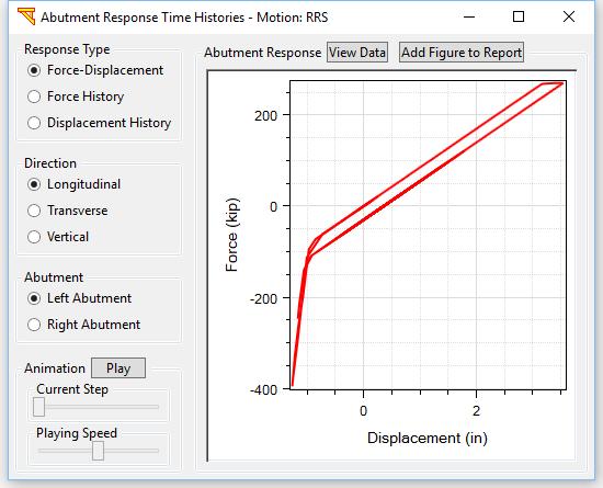
136 a) 118

137 b) Fig Abutment longitudinal force-displacement relationship: a) left abutment; and b) right abutment Soil Spring Responses Time Histories The soil spring responses can be accessed by clicking menu Display and then Soil Spring Response Time Histories. The soil spring responses window includes the following options (Fig. 114): i) Force-Displacement Curve ii) Displacement Time History iii) Force Time History Two directions (longitudinal and transverse directions) of the above responses for each soil spring are all displayed (Fig. 114). 119

138 Fig Soil spring response time histories Deck Hinge Responses Time Histories The deck hinge responses can be accessed by clicking menu Display and then Deck Hinge Response Time Histories. The deck hinge responses window includes the following options (Fig. 115): i) Force-Displacement Curve ii) Displacement Time History iii) Force Time History Response time histories are shown for the cable and edge hinge elements for each hinge (Fig. 115). 120

139 a) b) Fig Deck hinge response time histories: a) cable element; b) edge element 121

140 8.1.8 Isolation Bearing Responses Time Histories The isolation bearing responses can be accessed by clicking menu Display and then Isolation Bearing Response Time Histories. The isolation bearing responses window includes the following options (Fig. 116): i) Force-Displacement Curve ii) Displacement Time History iii) Force Time History Three translational directions and three rotational directions of the above responses for each bearing are displayed (Fig. 116). Fig Isolation bearing response time histories 8.2 Deformed Mesh and Animation The deformed mesh can be accessed by clicking menu Display (Fig. 3) and then Deformed Mesh. The deformed mesh window is shown in Fig

141 Analysis stages include Due to gravity anddue to pushover (or Due to base shaking). The response types include i) Deformed mesh ii) Resultant Disp. iii) X-Displacement iv) Y-Displacement v) Z-Displacement vi) Plastic Hinges In the Ground Shaking Analysis, the input motion is also animated at the deformed mesh window along with bridge displacement (Fig. 117). Fig Deformed mesh Visualization of plastic hinges is available if the nonlinear beam-column element is used for the columns. In the Ground Shaking Analysis, the input motion is also animated at the deformed mesh window along with the development of plastic hinges (Fig. 118). In the 123

142 current version, the visualization is implemented in such a way that a plastic hinge marker stays once the plastic hinge is developed. The plastic hinge is developed when rebar fails in tension or first concrete fiber reaches the maximum strain capacity. Fig Visualization of Plastic Hinges 8.3 Maximum Output Quantities EDP Quantities At the end of the finite element analysis phase, the following output EDP quantities (for each earthquake record) are available: 124

143 Table 6. Engineering Demand Parameters (EDP) EDP # EDP names 1 Maximum column drift ratio 2 Residual column drift ratio 3 Maximum relative deck-end/abutment displacement (left) 4 Maximum relative deck-end/abutment displacement (right) 5 Maximum bridge-abutment bearing displacement (left) 6 Maximum bridge-abutment bearing displacement (right) 7 Approach residual vertical displacement (left) 8 Approach residual vertical displacement (right) The EDP outcomes can be shown against the input base shaking IMs. The sections below detail how the response quantities are obtained for each EDP for the annotated model that is used to describe the location of sampling points during time history analysis. EDP1: Maximum drift ratio SRSS (column) EDP2: Residual drift ratio SRSS (column) The Square Root of Sum of Squares (SRSS) values of the 2 horizontal components are used. The drift ratios are combined separately at each time step (to obtain SRSS). EDP1 (Max drift ratio SRSS) is the maximum of the SRSS values of all time steps. EDP2 (Residual drift ratio SRSS) is the SRSS value at the last time step. The drift ratio is in percentage. EDP3: Maximum longitudinal relative deck-end/abutment displacement (left) EDP4: Maximum longitudinal relative deck-end/abutment displacement (right) These two EDPs are intended to address the issue of abutment impact into the backwall, so they are defined as only the motion of the deck into the abutment. Maximum absolute values in the longitudinal direction are used. EDP5: Maximum absolute bearing displacement (left abutment) EDP6: Maximum absolute bearing displacement (right abutment) These two EDPs are intended to address bearing damage whether or not an explicit representation of the bearings is included in the user-selected abutment model. Therefore, the EDP for the EDP is based on the relative displacements of the deck-end node to the abutment top node. The SRSS values of the resulting two relative horizontal 125

144 displacements is used and both motion into the backwall and away from the backwall are considered. EDP7: Residual vertical displacement (left abutment) EDP8: Residual vertical displacement (right abutment) This EDP is used to gage immediate repairs for rideability, and is not a measure of the permanent slumping of the embankment (for example). Therefore, the EDP is calculated as the vertical displacement of the abutment top node relative to the deck-end node. The residual value is used (value at the final time step). The EDP quantities for all input motions can be accessed by clicking menu Display (Fig. 3) and then EDP Quantities for All. The window to display EDP quantities is shown in Fig The EDP quantities are displayed against any of the 11 intensity measures. The EDP quantities for each input motion are displayed by bin of the motion (see legend in Fig. 119). When an IM is paired with an EDP and all the individual realizations are plotted, the result is typically termed a demand model, or probabilistic seismic demand model (PSDM). Fig EDP quantities for all motions 126

145 8.3.2 Bridge Peak Accelerations & Displacements for All Motions The bridge peak accelerations and displacements for all input motions can be accessed by clicking menu Display (Fig. 3) and then Bridge Peak Accelerations& Displacements for All Motions. The window to display the bridge peak accelerations for all motions is shown in Fig The responses are available in the longitudinal and transverse directions as well as for the SRSS of the 2 horizontal directions (Fig. 120). The figures in this window include: i) Maximum bridge acceleration ii) Maximum bridge displacement iii) Bridge peak acceleration / input peak acceleration a) 127

146 b) Fig Bridge peak accelerations for all motions: a) maximum bridge accelerations; b) maximum bridge displacements Maximum Column & Abutment Forces for All Motions The maximum column & abutment forces for all input motions can be accessed by clicking menu Display (Fig. 3)and then Maximum Column & Abutment Forces for All Motions. The window to display the maximum column & abutment forces for all motions is shown infig The responses are available in the longitudinal and transverse directions as well as for the SRSS of the 2 horizontal directions (Fig. 121). The figures in this window include: i) Maximum column shear forces ii) Maximum column bending moments iii) Maximum abutment forces (left abutment) iv) Maximum abutment forces (right abutment) 128

147 Fig Maximum column & abutment forces for all motions 129

148 9 EQUIVALENT STATIC ANALYSIS Equivalent Static Analysis (ESA) option is available in MSBridge for the bridge longitudinal & transverse directions. The whole bridge system is employed in the bridge longitudinal ESA. And one single bent is employed in the bridge transverse ESA. 9.1 Bridge Longitudinal Direction To conduct an Equivalent Static Analysis (ESA) for the bridge longitudinal direction, click Longitudinal Direction in the main window (Fig. 122). The elastic displacement demand output is shown in Fig The displacement demand output is available for the longitudinal components of the input motions. To view the comparison of displacements from ESA and Time History Analysis (THA), click Compare with THA. The comparison result is shown in Fig However, the comparison is only available for ESA for the longitudinal components of the input motions (Fig. 123). The procedure of the bridge longitudinal ESA is as follows: 1. Specify a load F of the total weight (see below for now to calculate the total weight), do pushover and get a displacement d 2. Calculate the Stiffness K = F/d 3. Calculate the Period T = 2π sqrt(m/k) 4. From the spectral acceleration of the input motion, get Sa 5. Calculate Dd= M*Sa/K, and this is the elastic displacement demand. 6. Check the abutment displacement (Dd) compared to abutment yield displacement (Dy). If Dd/Dy<2, stop, Dd is the demand. If Dd/Dy> 4, set abutment spring to 0.1*its initial stiffness, recalculate the displacement demand (Dd). If 2 <Dd/Dy< 4, linearly interpolate abutment stiffness between its full and 0.1 values and ratios of 2 and 4, then recalculate the displacement demand. The whole bridge system is employed in the bridge longitudinal ESA. As such, the pushover load is applied at the bridge center along the bridge deck (longitudinal) direction. The total weight is equal to the total deck weight plus ½ column weight. The deck weight should be distributed weight over span elements (or applied to nodes by tributary length). Column weight applied at top column node or if more than one element is used per column, distributed to column nodes by tributary length. 130

149 9.2 Bridge Transverse Direction To conduct an ESA for the bridge transverse direction, click Transverse Direction in the main window (Fig. 122). The output is shown in Fig Only one single bent is employed in the bridge transverse ESA. As such, the pushover load is applied at the bent cap center along the bent cap direction (bridge transverse direction). The total weight is equal to the deck weight of left half span and right half span for the bent plus ½ column weight. Fig Equivalent Static Analysis for the bridge longitudinal & transverse directions 131

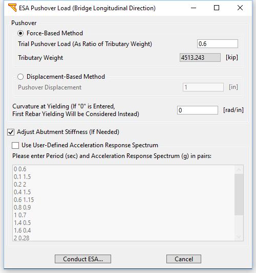
150 a) 132

151 Fig Sample output of ESA for the bridge longitudinal direction: a) pushover load; b) elastic displacement demand b) Fig Comparison of displacements from ESA and THA 133

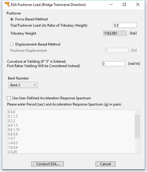
152 a) 134

153 b) Fig Output of ESA for the bridge transverse direction: a) pushover load and bent number; b) elastic displacement demand 135

154 10 PBEE ANALYSIS (GROUND SHAKING) To conduct a single earthquake analysis or a full PBEE analysis, the Ground Shaking option under Analysis Type (Fig. 2) is used. For that purpose, the input earthquake excitation(s) must be specified. Input files at that exercise this option include Examples 2-5. If only one earthquake record is selected out of a specified ensemble (suite) of input motions, then a conventional single earthquake analysis will be performed Theory and Implementation of PBEE Analysis In the user interface, an implementation of the Pacific Earthquake Engineering Research (PEER) Center s performance-based earthquake engineering framework (Cornell and Krawinkler, 2000) is used to generate probabilistic estimates of repair cost and repair time. The PEER PBEE framework utilizes the total probability theorem to compute the desired probability distributions by disaggregating the task into several intermediate probabilistic models with different sources of randomness and uncertainty. The hazard model uses earthquake ground motion data to determine an intensity measure (IM). The demand model uses response from dynamic analysis to determine an engineering demand parameter (EDP). The damage model connects the EDP to a damage measure (DM). Then, the DM is linked to consequences that are termed the decision variables (DV). Repair cost and repair time can be thought of as two possible decision variable (DV) outcomes characterized probabilistically by the framework. The complete analysis is accomplished using the local linearization repair cost and time methodology (LLRCAT), described by Mackie et al. (2010) and depicted conceptually in Fig In the LLRCAT methodology, each bridge system is disaggregated into independent structural or non-structural components or subassemblies defined as performance groups (PGs) that are damaged, assessed, and repaired together using a specific combination of different repair methods. Demands on the bridge system (and components) are determined using 3D nonlinear time history analysis under multiplecomponent earthquake excitation. The damage in each of the PGs is characterized according to several discrete damage states (DSs) that are defined by distributions of critical EDPs. A feature of the LLRCAT implementation used is the introduction of a repair model between the original PEER abstraction of DM and DV. Jumping directly from DMs to repair costs is difficult to accomplish, because it skips over the details of repair design and the variability of cost and time estimating. Creating these two additional models makes it easier to implement a step-by-step procedure for defining the models. The repair model and cost model are created through the process of schematic design of repairs and estimating the costs of those designs. Different repair methods are employed for the various damage states of each PG or bridge component. The repair methods for each PG require a combination of several repair quantities (Qs). Repair quantities for all PGs are then combined with due consideration of the correlation between components. Repair costs (RC) are obtained through a unit cost (UC). Repair times (RT) are obtained through 136

155 a production rate (PR). The PRs are in terms of crew working days (CWD), representing one working day for a normal sized crew and can be combined later by construction management experts to obtain total site construction times. Fig Schematic procedure of the LLRCAT methodology for a single bridge component The characterization and visualization of the ground motion suites using different choices of IMs will be discussed in Section 7.1. The FEM, parameter selection, analysis options, and outcomes that generated EDPs were similarly covered in Section 3. The bridge is then broken down into performance groups (PGs) for each major bridge superstructure, substructure, and foundation component. Each performance group represents a collection of structural components that act as a global-level indicator of structural performance and that contribute significantly to repair-level decisions. Performance groups are not necessarily the same as load-resisting structural components. For example, non-structural components may also form a performance group, since they also suffer damage and contribute to repair costs. The notion of a performance group also allows grouping several components together for related repair work. For example, it is difficult to separate all of the individual structural components that comprise a seat-type abutment (shear key, back wall, bearings, approach slab, etc.) as they all interact during seismic excitation and their associated repair methods are coupled. Therefore, the abutment repair group incorporates the fact that repairs to the back wall require excavation of the approach slab. Performance groups also address the issue of potentially double counting related repair items. Some repair items require the same preparation work such as soil excavation. For example, both back wall repair and enlargement of an abutment foundation require at least 4 ft of excavation behind the back wall. If these repair items were in different PGs, then double counting the excavation would be a problem. Bundling these related repair methods within a PG allows for independent consideration of each PG. The correlation between repair items from the PGs is handled at the demand model level in the 137

156 methodology. A total of 11 PGs are considered: PG1: Max column drift ratio; PG2: Residual column drift ratio; PG3: Max relative deck-end/abutment displacement (left); PG4: Max relative deck-end/abutment displacement (right); PG5: Max bridge-abutment bearing displacement (left); PG6: Max bridge-abutment bearing displacement (right); PG7: Approach residual vertical displacement (left); PG8: Approach residual vertical displacement (right); PG9: Abutment residual pile cap displacement (left); PG10: Abutment residual pile top displacement (right); PG11: Column residual pile displacement at ground surface. Discrete DSs are defined for each PG. Damage states are numbered sequentially in order of increasing severity. The DS0 damage state corresponds to the onset of damage when repair costs begin to accumulate. An upper limit to the quantities and costs is called DS, because it corresponds to the most severe possible damage state for the elements in a PG. DS usually corresponds to complete failure and replacement of all the elements in the entire PG. The DSs are connected to structural demands obtained from finite element analysis results by way of an EDP specific to each PG. The repair quantities associated with each DS are developed more fully in the definition of the damage scenarios. All the PGs and DSs are linked to a single EDP in this implementation. Based on previous work, the methodology was calibrated for defining post-earthquake performance of select bridges that fall within the class of ordinary post-tensioned, box girder, reinforced concrete highway overpasses (Mackie et al. 2011). The three major components required for this calibration were damage scenarios that describe particular instances of earthquake damage, schematic design of bridge repairs to address the state of damage in the scenarios, and the link between repair design, methods and procedures, and subsequent quantities. There is a direct link between damage scenarios and the repair, i.e., there is a single repair procedure for a single state of damage. The repair quantity results were parameterized in terms of basic bridge geometry and properties so that they can be used to extrapolate loss modeling for other bridges in the same class (such as those that can be built within the user interface). Data for time and monetary repair costs were obtained by estimating the costs of the damage and loss scenarios using published Caltrans construction estimation data, case studies from previous earthquakes, and interviews with Caltrans bridge engineers. Monetary costs were adjusted to 2007 values based on Caltrans cost index data. Repair costs are estimated for each damage scenario based on quantities of each repair item. Cost estimates accounted for variations in unit cost, and the details involved in estimating a combination of repairs together. The benefit of separating the Qs from costs is that the unit cost model is easily updated for new years of data, local economic conditions, site accessibility, and incentives. Normalized costs of repair are obtained by using the repair cost ratio (RCR) between the cost of repair and the cost of replacement cost (does not include demolition). It is shown in %, and it can range between 0 and some number higher than 100% (there is no reason why it is bounded by replacement cost; this is purely an owner/operator decision). This ratio is useful for comparing the performance of different bridge design options for new 138

157 construction. For the evaluation of existing structures, the RCR including demolition costs might be more useful. Constructing a new bridge on the same site after an earthquake would require both demolition of the damaged bridge and construction of its replacement. The costs of new construction used in the interface come from Caltrans bridge cost estimates used for planning purposes. They are based on the deck and type of construction, providing a range of cost/sf of deck area, circa 2007 to be consistent with the repair data used. Repair time for the bridge can be expressed either as an approximation of repair duration or repair effort. The repair effort represents the total number of crew-workdays (CWD) required to complete the task. This is different from repair duration, which counts the total duration of the repair project. The repair duration includes the effect of scheduling concurrent on-site construction processes, while the repair effort does not. The repair duration can vary based on the amount and type of concurrent construction processes, schedule dependencies, availability of labor, and whether or not contract incentives are provided in order to decrease duration. Repair times are also computed on the basis of each repair quantity Q. For any repair item, a probability of 50% that Q > tolerance indicates that the associated repair time should be added to the total repair time for the project (the tolerance is set at a value of 3% of Qn,max) Input Necessary for User-defined PBEE Quantities If the user is interested in providing user- or project-specific information in a PBEE analysis, the following paragraphs describe the data needed by the interface to execute the PBEE analysis and post-process the results. Performance groups need to be defined for each important component or subassembly of the system that has potential repair consequences. Performance groups are defined in terms of a single EDP that characterizes the response of this PG. Once this EDP metric has been defined and time history analysis performed to obtain a distribution of EDP realizations for different ground motions, the PBEE methodology can be implemented. The PBEE methodology requires definition (by the user) of discrete damage states for each PG, a repair method with associated repair quantities for each discrete DS for each PG, and the corresponding costs and times required to execute the repair method. The damage states are discrete and supplied in the form of what is commonly called a fragility curve. This is a misnomer however, because the information required is the value of the EDP (not IM) required to trigger different probabilities of exceeding the given discrete DS. It is often assumed that said curves are well described by the lognormal probability distribution and therefore, the only parameters required are the two lognormal distribution parameters: lambda and beta. Lambda is the median and beta is the lognormal standard deviation. A PG can have as many discrete DS as are required to cover the full range of possible responses experienced by the PG. These should be input as is shown in Section below. Once the different states of damage have been established, damage scenarios need to be generated that show different possible snapshots of damage that the structure may be in 139

158 after an earthquake event. Once these scenarios have been generated (note the scenarios need to be detailed and include exact descriptions of the extent and depth of damage), they can be used to decide what repair method would be appropriate for each PG or group of PGs. Such information is specific to the type of structure, the discrete DSs, and the PGs. It is really only obtainable from experts with past experience designing repair procedures given a damage scenario or snapshot. Once the repair methods have determined, specific details about the repair quantities (specific meaning square footage of deck, cubic yards of concrete, etc.) can be specified. The current data employed in the interface has repair quantities parameterized in terms of the common bridge design and geometric parameters, making it possible to solve for a variety of bridges within class. However, any changes beyond these configurations would require numerical values for all the repair quantities to be input. It is assumed that the repair quantity estimates for each PG and DS are also random quantities and can be described by a mean (or median) value and a coefficient of variation or lognormal standard deviation. In the interface, beta has been set as 0.4, but could be modified by the user in the future (if so desired). The repair quantities may then be handed over to a cost estimator, who would have the ability to access historical pricing and bid information. In addition, the type and magnitude of each repair quantity would correspond to standard DOT estimates and specifications procedures. Each repair quantity can then be bid or an estimation of cost and effort/time/production rate made. These unit costs and production rates are also random quantities and can be described by a mean (or median) value and a coefficient of variation or lognormal standard deviation. The values currently in the interface all have a beta of 0.2, but could again be set by the user if desired. See more details about PERT criteria for the production rates in Mackie et al. (2008). Modifying the default PBEE quantities (repair quantities, unit costs, and production rates) is detailed in Appendix E Definition/specification of PBEE input motion ensemble (suite) Available Ground Motions Four ground motion data sets are available: Motion Set 1: This PBEE motion ensemble were obtained from the PEER NGA database ( and consist of 100 3D input ground motions triplets, sorted into 5 bins. Each motion is composed of 3 perpendicular acceleration time history components (2 lateral and one vertical). These motions were selected through earlier efforts (Gupta and Krawinkler, 2000; Mackie et al., 2007) to be representative of seismicity in typical regions of California. The motions are divided into 5 bins of 20 motions each with characteristics: i) moment magnitude (Mw) and closest distance (R) km, ii) Mw and R km, iii) Mw and R km, iv) Mw and R km, and v) Mw and R 0-15 km. The engineering 140

159 characteristics (IMs and time histories) of each motion and of the ensemble overall may be viewed directly within BridgePBEE. Motion Set 2: These motions (160 in total) are developed by Dr. Mackie from the 80 motions of Motion Set 1 (excluding the 20 motions in bin v) above), to account for the more accurate site classifications (NEHRP C and NEHRP D) in NGA. The magnitude, distance, and spectral shape were intended to be similar to the previous bins (and indeed all of the previous motions appear in either the NEHRP C or NEHRP D bins now). As such, these motions are divided into 8 bins (compared to the 4 bins of Motion Set 1). Motion Set 3: These motions (80 in total) are labeled Broadband_* (separated into the two bins, Broadband rock and Broadband soil) as developed by Dr. Jack Baker for PEER. Additional information about these motions is available at the website: Motion Set 4: These motions (260 in total) include the above Motion Set 2 and Motion Set 3 as well as the additional bin v.) (near fault motions) of Motion Set 1. All of the above 4 ground motion data sets were resampled to a sampling frequency of 50 Hz (regardless of whether initial sampling frequency was 100 or 200 Hz) due to the computational demands of running full ground-structure analyses for an ensemble of motions. Standard interpolation methods were used to resample the time domain signals (so that the signal shape is preserved). The resampled records were then baselined to remove any permanent velocity and displacement offsets. Baselining was accomplished using a third order polynomial fitted to the displacement record Specifications of PBEE Input Motions To conduct a PBEE analysis, input motions must be defined (please follow the steps shown in Fig. 97). The window to define PBEE input motions is shown in Fig. 98. To unselect all motions, click De-select All. To see all motions, click Select All (same button as De-select All). The dropdown list of Randomly Choose Records for Each Bin will randomly select a certain number of input motions from each bin (the input motions are categorized by bin). Double-click any record to view its intensity measures and response spectra (Fig. 101). SRSS stands for Square Root of Sum of Squares of the 2 horizontal components. Click Display Intensity Measures (Fig. 98) to view the histogram and cumulative distribution plots for whole input motion set (Fig. 102). The intensity measures include: PGA (Peak Ground Acceleration) PGV (Peak Ground Velocity) PGD (Peak Ground Displacement) D5-95 (Strong Motion Duration) CAV (Cumulative Absolute Velocity) Arias Intensity 141

160 SA (Spectral Acceleration; assuming 1 second period) SV (Spectral Velocity), SD (Spectral Displacement) PSA (Pseudo-spectral Acceleration) PSV (Pseudo-spectral Velocity) The strong motion duration (D5-95) is defined according to the time domain bounded by the 5% and 95% cumulative Arias intensity of the record. All of the spectral intensity measures are defined at an effective viscous damping of 5% unless otherwise noted. In the histogram window (Fig. 102), click Display Intensity Measures Values to view the intensity measures listed in text format (Fig. 131). The user can copy and paste to her/his favorite text editor such as MS Excel (in Fig. 131, right-click and then click Select All to highlight, and then right-click and then click Copy to copy to the clipboard). To incorporate user-defined input motions, please see Appendix C. Step 1: click Ground Shaking. Step 2: click Select Input Motions. Fig Steps to define PBEE motions 142

161 Fig PBEE input motions widow 143

162 Fig Intensity measures of individual record (a) 144

163 (b) Fig (a) Histogram and (b) cumulative distribution for the whole input motion set 145

164 Fig Intensity Measures (IM) table for the whole input motion set 10.4 Save Model and Run Analysis After defining the finite element model, click on Save model and run analysis. The finite element computations will start, for several earthquakes at a time as specified in Fig. 128, the user can select as many as 8 records to be run at the same time in order to reduce the overall run time (for dual core machines or better). Fig. 104 shows the analysis progress for each record PBEE Analysis Once the FE analysis of all motions in the ensemble is complete, click PBEE Analysis (Fig. 2) to display: 146

165 Fig PBEE analysis window PBEE Quantities In the figure above (Fig. 132), under Damage States ( Fig. 133), Lambda is the median EDP that defines onset of the damage state and is one parameter of the assumed lognormal distribution of damage when conditioned in EDP. It has the same units as the EDP for the selected PG. Beta is the lognormal standard deviation and is the second parameter of the assumed lognormal distribution. Hence beta is dimensionless and has a typical range between 0 and 1 (although it is not bounded by 1). This parameter is closely related to the coefficient of variation (standard deviation normalized by the mean) under certain conditions (small beta values). In addition, the Repairs, Unit Costs, and Production Rates are displayed in Figs , respectively. 147

166 Fig Damage states window Fig Repair quantities window 148

167 Fig Unit Costs window 149

168 Fig Production Rates window Compute Repair Cost & Time Now, you can select any of the Intensity Measures (e.g., PGV above), and then click Compute Repair Cost or Compute Repair Time in Fig. 132 to display the probabilistic repair cost and Crew Working time in Days (CWD) along with Standard Deviation, displayed for each PG (eleven of them) and each repair quantity (29 of them, see Table 7), as shown below. See Section for the detailed output. To convert all PBEE figures to the EPS format, click Click Here for EPS Version of All PBEE Figures. A MS Word window with the EPS figures included in the document will 150

169 pop up once the converting is done (please see Section Error! Reference source not f ound. for the detailed output). Table 7. PBEE Repair Quantities Item# Item name 1 Structure excavation 2 Structure backfill 3 Temporary support (superstructure) 4 Temporary support (abutment) 5 Structural concrete (bridge) 6 Structural concrete (footing) 7 Structural concrete (approach slab) 8 Aggregate base (approach slab) 9 Bar reinforcing steel (bridge) 10 Bar reinforcing steel (footing, retaining wall) 11 Epoxy inject cracks 12 Repair minor spalls 13 Column steel casing 14 Joint seal assembly 15 Elastomeric bearings 16 Drill and bond dowel 17 Furnish steel pipe pile 18 Drive steel pipe pile 19 Drive abutment pipe pile 20 Asphalt concrete 21 Mud jacking 22 Bridge removal (column) 23 Bridge removal (portion) 24 Approach slab removal 25 Clean deck for methacrylate 26 Furnish methacrylate 27 Treat bridge deck 28 Barrier rail 29 Re-center column Compute Hazard Curves The user is also able to specify a Seismic Hazard for a particular geographic location of this bridge system in terms of specified values for any IM (e.g., derived from USGS seismicity maps). The user interface provides default values for site hazard specific to a location in Northern California. The hazard values are provided at each of the 2%-, 5%-, and 10%-probability of exceedance in 50 years only for PGA and PGV. The user should input hazard values specific to the site being studied as well as the intensity measure selected for analysis. If an IM other than PGA or PGV is selected, the user interface will 151

170 leave the three hazard level input boxes blank for user input as there are no readily available hazard maps or conversions from PGA for an arbitrary IM. The default PGA hazard values were obtained from USGS hazard maps. These PGA values were converted to PGV values using the firm ground conversion of 48 in./sec/g. It is not meant to imply that switching between PGA and PGV (or any other IM) will yield equal hazard. Once a desired local site seismicity is defined, users can click Display Hazard Curves (Fig. 132) to display the mean annual frequency of exceedance and return period. Please see Section for the detailed output Compute Disaggregation Users can also click Display Disaggregation (Fig. 132) to display the disaggregation by performance groups and repair quantities. Please see Section for the detailed output. Only the disaggregation of the expected repair cost/time by performance group is possible due to the LLRCAT formulation. However, both expected and variance disaggregation plots are available when disaggregating by repair quantity. The user can select the intensity measure and value on which to disaggregate. The default value is a PGV value equal to the 10% probability of exceedance in 50 years specified in the previous section. 152

171 11 TIME HISTORY AND PBEE OUTPUT 11.1 Time History Output Quantities At the end of the FE analysis phase, time histories and bridge responses will be available of the form: v) Column Response Time Histories and Profiles vi) Column Response Relationships vii) Abutment Responses viii) Deformed Mesh In addition, for PBEE analysis scenarios, Intensity Measures (IMs) and response spectra for each input motion are calculated and are available for display in Table and Figure formats. Performance Group (PG) Quantities and Bridge peak accelerations for all employed shaking motions are also available for display against any of the computed IMs. The post-processing capabilities can be accessed from Menu Display (Fig. 3). Fig. 137 and Fig. 138 show the post-processing capabilities available in a pushover analysis and a base shaking analysis, respectively. To display output for a different input motion, please follow steps shown in Fig The name of the selected input motion will also appear on the menu items (Fig. 138). Fig Post-processing capabilities (menu options) available in a pushover analysis 153

172 Fig Post-processing capabilities (menu options) available in a base shaking analysis a) 154

173 b) Fig Steps to display output for a different input motion: a) click menu Display (Fig. 3); b) select an input motion 11.2 PBEE Output Quantities At the end of the finite element analysis phase, the following output performance group quantities (for each earthquake record) are used in the next phase of PBEE analysis: Table 8. PBEE Performance Groups Performance Group Performance group names (PG) # 1 Maximum column drift ratio 2 Residual column drift ratio 3 Maximum relative deck-end/abutment displacement (left) 4 Maximum relative deck-end/abutment displacement (right) 5 Maximum bridge-abutment bearing displacement (left) 6 Maximum bridge-abutment bearing displacement (right) 7 Approach residual vertical displacement (left) 8 Approach residual vertical displacement (right) 9 Abutment residual pile cap displacement (left) 10 Abutment residual pile top displacement (right) 11 Column residual pile displacement at ground surface In addition, Intensity Measures for the computed Free Field ground surface acceleration records are computed, so that outcomes can be either shown against the input base shaking IMs or the computed ground surface IMs (noted as Free-Field in the user interface). The sections below detail how the response quantities are obtained for each PG. PG1: Maximum tangential drift ratio SRSS (column) PG2: Residual tangential drift ratio SRSS (column) The tangential drift ratio is defined as the maximum of a) displacement above the inflection point divided by the length of this distance, and b) displacement below the 155

174 inflection point divided by the length of this distance. This takes care of rotation at the base, different boundary conditions, etc., so that the results are consistent when computing damage. The Square Root of Sum of Squares (SRSS) values of the 2 horizontal components are used. The tangential drift ratios are combined separately at each time step (to obtain SRSS). PG1 (Max tangential drift ratio SRSS) is the maximum of the SRSS values of all time steps. PG2 (Residual tangential drift ratio SRSS) is the SRSS value at the last time step. The tangential drift ratio is in percentage. To calculate the tangential drift ratio, the following 2 lines were added into the tcl file: recorder Element -file A-ELC.dft -time -ele $columnele tangentdrift recorder Element -file A-ELC.ifp -time -ele $columnele inflectionpoint where $columnele is the element # of the column (Only one forced-based beam-column element nonlinearbeamcolumn is used for the column). In the.dft file, there will be 5 columns of data for each time step and the first column is time. In the.ifp file, there will be 3 columns for each time step and the first column is also time. Subsequently, the tangential drift ratio is calculated using the code snippet shown in Fig For the tangential drift ratio in the longitudinal direction (X-direction or bridge longitudinal direction), the tdx1 and tdx2 variables are the second and third column (the first column is time), respectively, of the tangential drift recorder file (e.g., A-ELC.dft). The tdxi variable is the second column (the first column is time) of the inflection point recorder file (e.g., A-ELC.ifp). For the transverse tangential drift ratio, the tdx1 and tdx2 variables are the fourth and fifth column of the.dft file and the tdxi variable is the third column of the.ifp file. // tdx1 & tdx2 -- the tangent drift recorder file at time step i // tdxi -- the inflection point recorder at time step i // tdx tangential drift ratio if( fabs(tdxi) < 1e-20 ) { tdx = -tdx2/(h - tdxi); } else if ( fabs(h-tdxi) < 1e-20 ) { tdx = -tdx1 / tdxi; } else { tdx = max(fabs(tdx1/tdxi), fabs(tdx2/(h-tdxi))); //tdx = -tdx*sgn(tdx2/(h-tdxi)); if( fabs(tdx2/(h-tdxi)) < 1e-20 ) tdx = 0; else if( (tdx2/(h-tdxi)) > 0) tdx = -tdx; } return tdx; Fig Code snippet to calculate the tangential drift ratio of column 156

175 PG3: Maximum longitudinal relative deck-end/abutment displacement (left) PG4: Maximum longitudinal relative deck-end/abutment displacement (right) These two PGs are intended to address the issue of abutment impact into the backwall, so they are defined as only the motion of the deck into the abutment. Maximum absolute values in the longitudinal direction are used. For example, for the right abutment, it is the relative longitudinal displacement of node B (deck-end node) in the direction of node C (abutment top node). A zero value is used for the times during which the deck-end node moves away from the abutment top node. PG5: Maximum absolute bearing displacement (left abutment) PG6: Maximum absolute bearing displacement (right abutment) These two PGs are intended to address bearing damage whether or not an explicit representation of the bearings is included in the user-selected abutment model. Therefore, the EDP for the PG is based on the relative displacements of the deck-end node to the abutment top node. The SRSS values of the resulting two relative horizontal displacements is used and both motion into the backwall and away from the backwall are considered. PG7: Residual vertical displacement (left abutment) PG8: Residual vertical displacement (right abutment) This PG is used to gage immediate repairs for rideability and is not a measure of the permanent slumping of the embankment (for example). Therefore, the EDP is calculated as the vertical displacement of the abutment top node relative to the deck-end node. The residual value is used (value at the final time step). PG9: Residual pile cap displacement SRSS (left abutment) PG10: Residual pile cap displacement SRSS (right abutment) These PGs address possible damage below grade due to lateral translation of the piles and pile caps. While not a direct measure, pile cap displacement was selected as it would not require knowledge or observations of piles below grade. The EDP is defined by calculating the SRSS value of the 2 horizontal displacements of the abutment pile cap node. The residual is obtained from the value at the final time step. PG11: Residual pile cap displacement SRSS (column) This quantity is analogous to the two previous PG but is representative of response and damage at the abutment foundations. The EDP is obtained by calculating the SRSS value of the 2 horizontal displacements of the column pile cap node and taking the value at the final time step. 157

176 The PG (Performance Group) quantities for all input motions can be accessed by clicking menu Display (Fig. 3) and then PG Quantities for All Motion (Fig. 141). The window to display PG quantities is shown in Fig The PG quantities are displayed against any of the 22 intensity measures (including 11 for the input acceleration and the other 11 for the free-field response). The PG quantities for each input motion are displayed by bin of the motion (see legend in Fig. 119). When an IM is paired with an EDP and all the individual realizations are plotted, the result is typically termed a demand model, or probabilistic seismic demand model (PSDM). Previous research has demonstrated that the central values of PSDMs are often well described using a power-law relationship between EDP and IM. The parameters of such a power-law fit can be obtained using least squares analysis on the data. Therefore, when plotted in log-log space (as is shown in Fig. 119), the best-fit, or mean, relationship is linear. The mean (in log-log space) is shown along with the standard deviation (also in log-log space) of the power-law fit. If it is assumed that the EDP responses are lognormally distributed when conditioned on IM, then these curves can be interpreted as being defined by the two parameters of a lognormal distribution (the median can be related to the mean of the logarithm of the data and the lognormal standard deviation is as shown). Fig Menu items to access the PG quantities for all motions 158

177 Fig PG quantities for all motions 159

178 11.3 PBEE Outcomes Repair Cost & Time The final PBEE results will be displayed against any intensity measure (e.g., PGV) in terms of: Contribution to expected repair cost ($) from each performance group (Fig. 143) Total repair cost ratio (%) (Fig. 144) Contribution to expected repair cost ($) from each repair quantity (Fig. 145) Contribution to repair cost standard deviation ($) from each repair quantity (Fig. 146) Total repair time (CWD) where CWD stands for Crew Working Day (Fig. 147) Contribution to expected repair time (CWD) from each repair quantity (Fig. 148) Fig Contribution to expected repair cost ($) from each performance group 160

179 Fig Total repair cost ratio (%) as a function of intensity Fig Contribution to expected repair cost ($) from each repair quantity 161

180 Fig Contribution to repair cost standard deviation ($) from each repair quantity Fig Total repair time (CWD: Crew Working Day) as a function of intensity 162

181 Fig Contribution to expected repair time (CWD) from each repair quantity Hazard Curves Based on the local site Seismic Hazard specified, losses are estimated and displayed graphically as: The defined local site hazard curve as a mean annual frequency ( ) of exceedance (ground motion) (Fig. 149) Return period against total repair cost ratio (Fig. 150) Mean annual frequency (MAF) of exceedance (loss) against total repair cost ratio RCR (Fig. 151) Return period against total repair time RT (Fig. 152) Mean annual frequency (MAF) of exceedance (loss) against total repair time (Fig. 153) The median ground motion hazard curve is assumed to have a power-law form with two unknown parameters (k, k0 in Eq. 4) in the range of the ground motion intensities bracketed by the 2%- and 10%-probability of exceedance IM values (im). The twoparameter fit (linear in log space) to the nonlinear (in log space) hazard curve tends to overpredict frequencies of exceedance for IM extremes both above and below the range of intensities considered. Therefore, care should be taken when extrapolating any resultant hazard curves to extremely low (or high) frequencies of exceedance. Using a least-squares fit in log space, the unknown parameters can be determined numerically from the three values input by the user (2%-, 5%-, and 10%-probability of exceedance in 163

182 50 years). On the site hazard curves plotted in the interface, both the data points and the fitted curve are shown (Fig. 149). I ( i M )=k m 0 ( i ) k m (4) The power-law fit to the hazard data is used to compute the loss hazards. The loss model (probability of exceeding RCR or RT conditioned on intensity levels) is integrated with the absolute value of the derivative of this IM hazard to obtain the loss hazard curve (MAF of exceeding either RCR or RT). Details of the numerical integration are presented in Mackie et al. (2008) and other sources. The loss hazard curves (both for repair cost and repair time) are further integrated over intensity to yield mean annual loss. For example, in Fig. 151, the mean annual repair cost ratio expected for the bridge at the given site is 0.05% of the replacement cost. Fig Mean annual frequency of exceedance (ground motion) 164

183 Fig Return period against total repair cost ratio 165

184 Fig Mean annual frequency of exceedance (loss) against total repair cost ratio 166

185 Fig Return period against total repair time 167

186 Fig Mean annual frequency of exceedance (loss) against total repair time Disaggregation Figs display the disaggregation (Fig. 132) of expected cost by performance group, the disaggregation of expected cost by repair quantities, and the disaggregation of expected time by repair quantities, respectively. In thie figures below, the disaggregation is performed at an intensity of 100 cm/s (PGV) for all three figures (a user IM and value as shown in Fig. 132). This IM and its value are shown in the plot titles. 168

187 Fig Disaggregation of expected cost by performance group 169

188 Fig Disaggregation of expected repair cost by repair quantities 170

189 Fig Disaggregation of expected repair time by repair quantities 171

190 APPENDIX A CAPABILITIES ADDED IN THE CURRENT UPDATED VERSION A number of capabilities and features have been added in the current version of MSBridge. These added features mainly allow MSBridge to address possible variability in the bridge deck, bent cap, column, foundation, and soil configuration/properties (on a bent-by-bent basis). Specifically, the capabilities implemented are: (a) A different skew angle can be defined for each individual bent/abutment (in MSBridge, from main window -> Advanced -> check Use Individual Skew Angles -> Bent and Abutments). (b) A different skew angle can be defined for each individual deck hinge (from main window -> Advanced -> Define Deck Hinges). (c) Shear key option (using OpenSees Bilin material) is included in the deck hinge model. The shear key is not activated by default (From main window -> Advanced -> Define Deck Hinges -> Modify). (d) Deck and bentcap are now connected by a rigid link (deck offset is activated in this case). A hinge with 6 Degrees of freedom (DOF s) of linear springs can be activated at the rigid link, at the location that the user specifies (From main window -> Bentcap). (e) Box girder section graphical representation has been added (for efficient incorporation of the user defined properties). (From main window -> Deck -> Recalculate Section from Box Girder) (f) Option to couple longitudinal and transverse directions of isolation bearing nonlinear response has been added (From main window -> Advanced -> Define Isolation Bearings -> Couple Longitudinal and Transverse Directions). (g) Definition of the bent cap properties is now allowed on a bent by bent basis (From main window -> Bentcap). (h) Definition of the column properties is allowed for each individual column. This option gives the user great flexibility and control over assigning different nonlinear fiber sections to columns and pile shafts (Types I & II), (From main window -> Column). (i) Oblong column cross section with two circular steel cages has been added (From main window -> Column -> Oblong). (j) For the circular cross section, options for Bonded and Un-bonded Column Jackets (i.e., Casing as Fibers in the Bonded case) have been added (From main window -> Column -> Circle -> check Activate Steel Jacket). 172

191 (k) Option to improve computational analysis schemes has been added. Specifically, this option is mainly to allow automatic switching between time integration schemes to achieve convergence in highly nonlinear scenarios (From menu Execute -> Advanced Option: OpenSees Parameters -> check Automatic Switching between Time Integration Schemes). Furthermore, the following options have been implemented: (a) Concrete properties can be manually specified (instead of automatically calculated from the column geometry and reinforcement information) (From main window -> Column -> check Update RC Properties and click Nonlinear Fiber Section). (b) Option to enter user-defined moment curvature (from main window -> Column -> check User-Defined Moment Curvature and click Define Moment Curvature). (c) A separate steel material can be used for the steel jacket (From main window -> Column -> Nonlinear Fiber Section). (d) Option to include the vertical soil springs for the Soil Springs foundation type (From main window -> Foundation -> click Soil Springs and then Modify Soil Springs). (e) Option to calculate the vertical soil springs (for the Soil Springs foundation type) based on user-defined T-z and Q-z data (From main window -> Foundation -> click Soil Springs and then Modify Soil Springs -> click Calculate from User T- z and Q-z). (f) Option to specify a yielding curvature as the yielding criterion for Longitudinal and Transverse ESA (From main window -> click Longitudinal Direction (or Transverse Direction). (g) A different number of columns can be specified for each individual bent, with locations defined by column offsets (From main window -> Bridge -> check Nonuniform Column Layout -> Columns). (h) Column base offset (zero by default) can also be defined, for modeling inclined columns (From main window -> Bridge -> check Non-uniform Column Layout -> Columns -> specify Base Offset). (i) Different deck properties can be specified on a span-by-span basis (From main window -> Deck; from main window -> Bridge -> check Non-uniform Column Layout). (j) For Horizontal Alignment, the global coordinate system can be rotated at the angle specified; or the bridge longitudinal direction can be chosen to coincide with the 173

192 chord connecting the two abutments (From main window -> Spans -> check Horizontal Alignment -> Modify Horizontal Curve). (k) Option to include the bentcap overhang (the portion of the bent cap outside the columns) has been added (From main window -> Bentcap). (l) Option to include the user defined TCL code snippet for the nonlinear Fiber section has been added. This is an advanced option and the users must proceed with caution (From main window -> Column -> check User-Defined Tcl Script for Nonlinear Fiber Section -> Define Fiber Section Tcl Script). (m) Different Foundation Matrix parameters can be assigned to each column base (From main window -> Foundation -> check Foundation Matrix -> Modify Foundation Matrix). (n) Option to include pile cap masses and fixity conditions has been added, available only in the foundation types Soil Springs and Foundation Matrix (From main window -> Advanced -> Pilecap Mass and Rotation Condition). (o) Option to include column P-Delta effect (included by default) has been added (From main window -> Advanced -> check/uncheck Include P-Delta Effect). (p) Option to include Rayleigh (stiffness proportional component) damping for the abutments has been added, with no Rayleigh damping for the abutment stiffness as the default (From main window -> Advanced -> check/uncheck Include Rayleigh Damping). (q) Deck-end fixity conditions can be directly applied (From main window -> Advanced -> Deckend Fixity) (r) Visualization of pile response (profiles, time histories and relationships) has been added, available for the foundation type Soil Springs (From menu Display -> Pile Response Profiles/Pile Response Time Histories/Pile Response Relationships). (s) Option to view OpenSees analysis log (From main menu -> Execute -> OpenSees Analysis Log). (t) Multi-Linear abutment model has been added (From main window -> Abutment -> select Elastic/Multi-Linear Abutment -> Modify Properties). (u) Option to include Rayleigh (stiffness proportional component) damping for the soil springs has been added, with no Rayleigh damping for the soil springs as the default (From main window -> Advanced -> check/uncheck Include Rayleigh Damping). 174

193 (v) Option to activate the linear behavior for the soil springs (From main window -> Advanced -> Linear Soil Springs). (w) Option to choose a beam column element type for pile shafts (From main window -> Mesh). 175

194 APPENDIX B CALCULATION OF STEEL AND CONCRETE MATERIAL PROPERTIES Steel Bars By default, the Steel02 material is used to simulate steel bars. The format of the Steel02 command is as follows (McKenna et al. 2010): uniaxialmaterial Steel02 $mattag $fy $E0 $b $R0 $cr1 $cr2 Where $fy is the steel yield strength, $E0 is Young s modulus of steel, and $b is the strain-hardening ratio (ratio between post-yield tangent and initial elastic tangent), $R0, $cr1 and $cr2 are parameters to control the transition from elastic to plastic branches. The number of longitudinal bars is calculated as follows: # s bars= Ac A b (5) s Where is the longitudinal steel percentage, Ac the column cross-section area, Ab is the cross-section area of the steel bar. If the number of longitudinal bars is known, the longitudinal steel percentage (reinforcement ratio) can be calculated: = s A A s c (6) Where As is the area of longitudinal steel, which is equal to the area of each bar times the number of bars. For example, the diameter of a #18 bar is inches, so area is 4 in 2. If there are 10 bars in a 36 inch diameter circular column, then s 10(4) = = or 3.9%. The transverse steel percentage (reinforcement ratio) for a spirally confined circular column, currently the only type of column supported in the interface, is ( d t = s( d 2 db cc ) ) (7) 176

195 Where dbt is the diameter of the transverse spiral (always smaller than the diameter of the longitudinal bars). The spacing between transverse bars is s. The diameter of the confined core is dcc which is the gross diameter minus twice the cover and minus the diameter of the transverse bars (see Eq. 10). So for a #5 spiral spaced at 3 inches on center in the same column mentioned above. t 5 2 ( ) = 8 = (36 2(2) ) 8 (8) or 1.3%. Currently the transverse reinforcement does affect the shear response (through changes in the uniaxial constitutive model for the concrete core). However, the columns are modeled considering only flexurally dominated response (i.e., there is no accounting for shear flexibility or shear degradation directly). Additional relevant details on the parameters used in both the Cover and Core Concrete are included below. Cover concrete The Concrete02 material is used to simulate the concrete (for both cover and core). The format of the Concrete02 command is as follows: uniaxialmaterial Concrete02 $mattag $fpc $epsc0 $fpcu $epsu $lambda $ft $Ets Where $fpc is the concrete compressive strength, $epsc0 is the concrete strain at maximum strength, $fpcu is the concrete crushing strength, $epsu is the concrete strain at crushing strength (all of the above values are entered as negative), $lambda is the ratio between unloading slope at $epsu and initial slope, $ft is the tensile strength, and $Ets is tension softening stiffness (absolute value) (slope of the linear tension softening branch). For cover concrete, $fpc is equal to the concrete unconfined strengtherror! Reference s ource not found., $epsc0 = 0.002, $fpcu = 0.0, $epscu = 0.006, $lambda = 0.1, $ft = (0.14)$fpc, and $Ets = $ft / $epsc0. Core concrete i) For core concrete of circular column cross sections according to the Mander model, the procedure to calculate the confined concrete strength $fpc(= ) is as follows: f cc f c ' ' ' ( f e f e c= f c ) ' f f ' c c (9) 177

196 ' ' Where f c is the unconfined compressive strength and f e can be obtained from the following equation: f ' e = 1 Ke t f 2 y (10) Where f is the steel yield strength, is the transverse steel percentage, and K e can be y obtained from the following equation for circular columns confined by hoops: t K e = S' (1 ) 2dcc (1 ) cc 2 (11) Where: cc A = A s cc (12) An assumed value of the area of the confined core is used for default values. This area should be modified based on the expected compressive block in the column during lateral loading. 2 ( dc ) c Ac c= (13) 4 S ' t 2 bt d = d cc (14) Where dbt is the transverse bar diameter d c c = D 2c d L b t (15) Where c is the clear cover (c = 1.5 ) ii) $epsc0 epsc0 = 2 f E cc c (16) Where: 178

197 Ec = 1.5 ' 0.043w f c (17) Where w is the concrete unit weight (unit: kg/m 3 ) iii) $epsu (= ) e p s c u epscu = s f f y ' c t (18) s s =.0 12 Where is the ultimate steel strain ( ) f cu iv) $fpcu (= ) Where: f cu = fcc ( epscu) ( epscr) ( ( epsc) ( epscu) ( epscr) 1+ ( ) ( epsc) (ep scr) ) (19) f cc epsc = ( epsc0)(1 + 5( 1)) ' f c (20) eps cr = E c E c f cc (eps c) (21) Notes: 1. The information above is specific to the Steel02 and Concrete02 models of the Fiber section. Other options include (Fig. 24), Steel01 and Concrete01 (for more information please see the OpenSees documentation), and Elastic properties for the fibers. These options can be activated by clicking on the default Steel02 or Concrete02 sections (Fig. 24) and changing these options. 2. A different property may be specified for the Column below grade (for instance to roughly represent a large pile group as a large single column). If this option is selected (Fig. 6), the column below grade will have linear properties as specified by its diameter and Young s Modulus). 179

198 3. All the equations presented in this Appendix are based on the Mander model for spiralreinforced circular concrete columns. The user may want to use their own constitutive model or parameters. In this case, the values of these parameter can be defined directly in Fig

199 APPENDIX C HOW TO INCORPORATE USER-DEFINED MOTIONS 1) Directory Structure of a Motion Set To conduct a base input acceleration analysis, input motions must be defined (Fig. 97). The window to define the input motions is shown in Fig. 98. Click Browse to select a motion set (Fig. 157). Click on the motion set name (e.g., Motions) and then click on OK to choose this motion set (Fig. 157). In MSBridge, the input motions are organized in a format that the program can read. Specially, the input ground motions are sorted into bins. Fig. 158 shows the directory structure of a motion set named Motions. The second level directories are bins (e.g., T01; see Fig. 157 and Fig. 158). The third level directories are earthquake names (e.g., there is earthquake NORTHRIDGE; see Fig. 158). And the fourth level directories are the input motion names (e.g., there is 1 input motion under earthquake NORTHRIDGE: RRS; see Fig. 158). Each motion is composed of 3 perpendicular acceleration time history components (2 laterals and one vertical). As shown in Fig. 158, each motion folder contains 6 files categorized into 2 file types: the DATA files contain the time history (acceleration unit in g) of a component and the INFO files contain the characteristics of the corresponding component. Fig. 159 and Fig. 160 displays sample INFO & DATA files. Naming of these files usually has to follow the format below: Input motion name + angle (or "-UP" or "- DWN" for vertical component) + ".AT2" + ".data" (or.info"). However, the following format is also allowed: Input motion name + "-E" or "-W" for horizontal components (or "-V" for vertical component). Note that the filenames with the smaller angle will be used for the longitudinal direction and the other one (with the larger angle) will be used for the transverse direction (also, the filenames containing "-E" will be used for the longitudinal direction and the other one (containing "-W") will be used for the transverse direction. The first 2 lines of each INFO file must follow the style of the example below: {Data points NPTS}{996} {Sampling period DT (sec)}{ } Where 996 and 0.02 are the number of data points, and the time step, respectively, of an input motion component. 2) Steps to Create an Input Motion Based on the above description for the directory structure of a motion set, one can easily create an input motion (Fig. 161): 181

200 Step 1: create a folder and rename to your motion set name (e.g. MotionSet1; see Fig. 161). Step 2: create a folder under the motion set folder and rename to your bin name (e.g., bin1). Step 3: create a folder under the bin folder and rename to your earthquake name (e.g., Quake1). Step 4: create a folder under the earthquake name and rename to your input motion name (e.g. MOTION1). Step 5: create the 6 files (3 INFO files and 3 DATA files) for this input motion (Fig. 161). Note: If you download the input motion files from the PEER NGA Database, there is no need to re-format the data into one column as shown in Fig Just copy the data points into the corresponding DATA files. And then make the INFO files containing the number of data points and the sampling period DT (2 lines) according to the header information. 182

201 Fig Choosing a motion set 183

202 Fig Directory structure of a motion set Fig Sample.info file 184

203 Fig Sample.data file Fig Example of user-defined motion 185