Essays on the Measurement of Subjective Well Being across Countries

Transcription

1 Essays on the Measurement of Subjective Well Being across Countries Cristina Sechel PhD University of York Economics September 2015

2 Abstract The use of Subjective Well-Being (SWB) data in Economics is growing rapidly. Although traditionally marginalized due to their subjective nature, several studies provide convincing evidence that SWB data are reliable and valid sources of well-being information, and can provide supplementary information to that obtained from standard objective indicators of well-being. The overarching aims of this thesis are to gain a deeper understanding of how SWB data can best be used to measure national SWB, and to explore the properties of life satisfaction data. This thesis proposes a new measure of national SWB, designed for use with highresolution SWB scales. The proposed measure is defined as the share of satisfied individuals and is constructed using reported life satisfaction data from the World Values Survey and the European Values Survey. It is argued that this headcount measure is better suited for use with SWB data, which are bounded, ordinal, and arbitrary. Satisfied individuals are identified using a data-driven approach based on an observed data-cliff in reported life satisfaction, and motivated by cognitive dissonance theory. The proposed theory suggests that the observed data-cliff indicates individuals reluctance to report below satisfaction level 5 (on a scale of 1-10). Regression analysis is used to explore the relationship between national life satisfaction and objective indicators of development. An important result is that the proportion of satisfied individuals is found to be strongly associated with social indicators of well-being (i.e. life expectancy and education measures) but not significantly associated with per capita Gross National Income. This thesis also attempts to identify the driving factors behind the observed datacliff. Individual-level multivariate analysis reveals that individuals are reluctant to report below satisfaction level 5 in response to a reduction in income, dropping trust levels, and failing health; but changes in employment and marital status tend to overcome this reluctance. 2

3 Table of Contents Table of Contents... 3 List of Figures... 5 List of Tables... 9 Acknowledgements Author s Declaration Chapter 1. Introduction Chapter 2. A Proposal for a Headcount-Based Subjective Measure of National Progress Introduction Background: Issues Surrounding Subjective Well-Being Reporting Distortions and True Subjective Well-Being Interpersonal Comparisons of Utility Subjective Well-Being and National Development A Literature Review The Value of Aggregate Measures A Headcount Measure of Satisfied Individuals Mean Measures of Subjective Well-Being A Practical Headcount Measure and Its Advantages Data Description Choosing a Threshold Level Alternative Cut-Off Choices and Advantages of a Data-Driven Approach Rank Comparisons Concluding Remarks Chapter 3. The Subjective-Objective Relationship across Countries: An Aggregate Analysis using the Share of Satisfied Individuals Introduction Data Sources and Description Data Matching The Analysis Dataset Econometric Model Conventional Baseline Specification Beta-regression Results A note on the interpretation of results

4 3.4.2 Ordinary Least Squares Linear Model Results Beta-regression Results Comparisons to Mean Satisfaction Data Comparability Considerations Unbalanced Panel Issues Data Comparability within Second Wave ( ) Concluding Remarks Chapter 4. Response Distribution of Life Satisfaction: an individual-level analysis Using Ordered Response Models Introduction Theory and Related Literature The scale of SWB data The satisfaction curve and the distribution of SWB data Data Econometric Specifications Results Ordinal Probit (OP) Regression Generalized Ordinal Probit (GOP) Concluding Remarks Chapter 5. Conclusion Appendix A Appendix B Appendix C Bibliography

5 List of Figures Figure 2.1. Dissonance level across the SWB path Figure 2.2. Distribution of satisfaction responses, by wave Figure 2.3. Rankings based on the share of satisfied individuals, various cut-offs ( ) Figure 2.4. Rankings based on the share of satisfied individuals, various cut-offs ( ) Figure 2.5. Country rank differences between rank B and rank A (both waves combined) Figure 2.6. Country rank differences between rank B and rank D (both waves combined) Figure 2.7. Life satisfaction in Canada and Mexico (both waves combined) Figure 3.1. Cultural map ( average) Figure 3.2. Subjective-objective data matching Figure 3.3. Aggregate satisfaction and per capita GNI, all countries (both waves combined) Figure 3.4. Distribution characteristics of aggregate satisfaction (both waves combined) Figure 3.5. Average marginal effects on the share of satisfied individuals in model (2b) at various values of ln(gni), with 95% confidence intervals Figure 3.6. Average marginal effects on mean satisfaction in model (3b) at various values of ln(gni), with 95% confidence intervals Figure 4.1. Individual satisfaction path and corresponding aggregate satisfaction distribution Figure 4.2. Distribution of satisfaction responses (all countries), kernel density with Gaussian function overlaid Figure 4.3. Annual household income response distribution for all countries pooled (full sample)

6 Figure 4.4. Distribution of income by health, education, marital status, and employment status Figure 4.5. Distribution of age by health, education, marital status, and employment status Figure 4.6. Distribution of the number of children by health, education, marital status, and employment status Figure 4.7. Predicted probabilities across satisfaction levels, with 95% confidence intervals (OP regression) Figure 4.8. Marginal effects of income across satisfaction levels with 95% confidence intervals (OP results) Figure 4.9. Changes in the probability distribution of life satisfaction responses in response to a decrease in income from its mean value Figure Marginal effects of trust across satisfaction levels with 95% confidence intervals (OP results) Figure Marginal effects of religiousity across satisfaction levels with 95% confidence intervals (OP results) Figure Marginal effects of bad health across satisfaction levels with 95% confidence intervals (OP results) Figure Marginal effects of good health across satisfaction levels with 95% confidence intervals (OP results) Figure Marginal effects of being married across satisfaction levels with 95% confidence intervals (OP results) Figure Marginal effects of being separated/divorced across satisfaction levels with 95% confidence intervals (OP results) Figure Marginal effects of being widowed across satisfaction levels with 95% confidence intervals (OP results) Figure Marginal effects of unemployment across satisfaction levels with 95% confidence intervals (OP results) Figure Distance between adjacent estimated cutpoints (OP regression) Figure Predicted probabilities across satisfaction levels, with 95% confidence intervals (GOP regression) Figure Marginal effects of income across satisfaction levels with 95% confidence intervals (OP and GOP results)

7 Figure Marginal effects of trust across satisfaction levels with 95% confidence intervals (OP and GOP models) Figure Marginal effects of religiousity across satisfaction levels with 95% confidence intervals (OP and GOP models) Figure Marginal effects of bad health across satisfaction levels with 95% confidence intervals (OP and GOP models) Figure Marginal effects of good health across satisfaction levels with 95% confidence intervals (OP and GOP models) Figure Marginal effects of being married across satisfaction levels with 95% confidence intervals (OP and GOP models) Figure Marginal effects of being separated/divorced across satisfaction levels with 95% confidence intervals (OP and GOP models) Figure Marginal effects of being widowed across satisfaction levels with 95% confidence intervals (OP and GOP models) Figure Marginal effects of unemployment across satisfaction levels with 95% confidence intervals (OP and GOP models) Figure A1. Life satisfaction distribution, (by country) Figure A2. Life satisfaction distribution, (by country) Figure B1. Mass value changes for countries with data points in both waves Figure C1. Distribution of satisfaction responses (original sample) Figure C2. Relative frequencies of responses, for full sample and the restricted sample excluding missing income Figure C3. Marginal effects at means and average marginal effects with 95% confidence intervals, for income (Ordinal Probit) Figure C4. Marginal effects at means and average marginal effects with 95% confidence intervals, for trust (Ordinal Probit) Figure C5. Marginal effects at means and average marginal effects with 95% confidence intervals, for religiousity (Ordinal Probit) Figure C6. Marginal effects at means and average marginal effects with 95% confidence intervals, for bad health (Ordinal Probit)

8 Figure C7. Marginal effects at means and average marginal effects with 95% confidence intervals, for good health (Ordinal Probit) Figure C8. Marginal effects at means and average marginal effects with 95% confidence intervals, for marriage (Ordinal Probit) Figure C9. Marginal effects at means and average marginal effects with 95% confidence intervals, for separation/divorce (Ordinal Probit) Figure C10. Marginal effects at means and average marginal effects with 95% confidence intervals, for being widowed (Ordinal Probit) Figure C11. Marginal effects at means and average marginal effects with 95% confidence intervals, for part-time employment (Ordinal Probit) Figure C12. Marginal effects at means and average marginal effects with 95% confidence intervals, for self-employment (Ordinal Probit) Figure C13. Marginal effects at means and average marginal effects with 95% confidence intervals, for unemployment (Ordinal Probit)

9 List of Tables Table 2.1. Examples of relevant SWB survey questions Table 2.2. Individual responses, by wave and survey initiative Table 2.3. Distribution of life satisfaction responses, by wave Table 2.4. Sample sizes for countries surveyed under both EVS and WVS Table 2.5. Sample size statistics for countries surveyed under EVS or WVS (but not both) Table 2.6. Spearman correlation coefficients for rankings at various cut-offs (by wave). 47 Table 2.7. Country rankings (wave ) Table 2.8. Country rankings (wave ) Table 3.1. United Nations development indicators Table 3.2. Macro-level socioeconomic measures Table 3.3. Summary statistics Table 3.4. Data and econometric models used in previous studies involving the use of SWB information in development Table 3.5. Variances decomposed Table 3.6. OLS coefficients with the share of satisfied individuals as dependent variable Table 3.7. Beta-regression marginal effects at means with the share of satisfied individuals as the dependent variable Table 3.8. Beta-regression marginal effects at means with mean satisfaction as the dependent variable Table 3.9. T-tests for differences in aggregate SWB between EVS and WVS samples for countries surveyed under both initiatives in wave Table 4.1. Measures of interest Table 4.2. Summary statistics for selected explanatory variables (individual-level and country-level means) Table 4.3. Frequency tables for ordinal and nominal explanatory variables, all countries pooled (full sample, and subsamples around data-cliff) Table 4.4. Subsample comparison with t-tests for differences in means

10 Table 4.5. Subsample comparison with χ2 tests for independence between subsamples Table 4.6. Pearson correlation coefficients for selected explanatory variables Table 4.7. Lambda coefficients for categorical variables Table 4.8. Ordered Probit results, marginal effects at means of regressors Table 4.9. Generalized Ordered Probit results, marginal effects at means of regressors. 143 Table A1. Additional measures of interest (WVS and EVS combined) Table A2. Distribution of responses for additional measures of interest Table A3. Spearman correlation coefficients, various country rankings (by wave) Table A4. Country rankings, (including rank based on Gini coefficient) Table A5. Country rankings, (including rank based on Gini coefficient) Table B1. Country availability classified by geographical controls (by wave) Table B2. Additional UNDP indicators Table B3. OLS coefficients with the share of satisfied individuals as dependent variable, models with different cultural indicators Table B4. OLS coefficients with mean satisfaction as dependent variable Table B5. Beta-regression marginal effects at means with mean satisfaction as the dependent variable (original mean satisfaction scale ranging 1-10) Table B6. OLS coefficients with the share of satisfied individuals as dependent variable (for subsample of countries appearing in both waves) Table B7. Beta-regression marginal effects at means with the share of satisfied individuals as the dependent variable (for subsample of countries appearing in both waves) Table B8. Beta-regression marginal effects at means with mean satisfaction as the dependent variable (for subsample of countries appearing in both waves) Table B9. Beta-regression coefficients with the share of satisfied individuals as the dependent variable Table B10. Variables used to construct the Inglehart and Welzel index of Traditional vs. Secular-Rational values Table B11. Variables used to construct the Inglehart and Welzel index of Survival vs. Self- Expression values

11 Table C1. Sample attrition due to missing information, by measure of interest Table C2. Sample sizes and attrition due to missing information, by country Table C3. Distribution of responses, original categories for select variables Table C4. Summary statistics for select variables, country-specific (all countries) Table C5. Frequency table for self-reported Health, country-specific (all countries) Table C6. Frequency table for Education, country-specific (all countries) Table C7. Frequency table for Marital Status, country-specific (all countries) Table C8. Frequency table for Employment Status, country-specific (all countries) Table C9. Cross-tabulations for categorical variables Table C10. Ordered Logit results, marginal effects at means of regressors

12 Acknowledgements Firstly, I would like to thank my supervisor, Professor Karen Mumford, for her invaluable support and guidance. I am sincerely grateful to her for her constant encouragement and suggestions. I am happy to have had such a caring and dedicated supervisor. I would also like to thank Professor Mozaffar Qizilbash for his suggestions and input as co-supervisor during the first 2 years of my PhD studies. I have learned much from our discussions and they have greatly helped shape my research path. I am very grateful to my TAP members, Dr. Giacomo De Luca and Dr. Maria Garcia Reyes, for their helpful suggestions and questions. I am also grateful to the Department of Economics and Related Studies at The University of York for granting me a Departmental PhD Studentship, without which I would have been unable to fully cover the tuition fees and complete my studies. To my partner Victor Bandur, who has been by my side for many years, I am profoundly grateful for the happiness and confidence he has given me. He has supported and inspired me each and every day, and I am a better person and researcher because of him. To my parents, I am forever thankful for their unconditional and unwavering support. To my fellow PhD student, Malgorzata Mitka, I am thankful for her warm friendship and continual encouragement. Her wonderful sense of humour has kept me working through long winter days. 12

13 Author s Declaration I hereby declare that this doctoral thesis is my own work and effort and has been carried out during my time as a PhD student at the University of York from October 2011 to September I am the sole author of all chapters included herein. I also declare that this thesis has never been submitted for any other degree at any other university or educational institution. The work contained here is original except for external sources of information which have been acknowledged and cited, and has not been previously published in full or in part. The views expressed here are my own. 13

14 Chapter 1. Introduction The well-being of individuals and societies has long been at the root of the study of Economics under the umbrella term utility. Utilitarianism, the theory that social welfare rests on the sumranking of individual utilities, has been advanced and supported by many leading economists, such as Bentham, Marshall, and Pigou 1. The concept of utility is now an underlying principle of modern economic theories, whether explicitly (e.g. consumer theory) or implicitly (e.g. development economics). Although foundational, utility has typically not been measured or quantified in Economics and Economists have generally resisted defining utility in more tangible terms. However, there is now a rapidly growing body of literature linking utility to Subjective Well-Being (SWB), and widespread interest in measuring and understanding SWB. There are several main branches of interest regarding the study of SWB in Economics. First, there is a strong focus on establishing the determinants of SWB (e.g. Bjornskov et al., 2008), and especially on measuring the relationship between income and SWB (Diener and Oishi, 2000). Second, there are efforts to identify and overcome measurement challenges which are relevant for self-reported data, such as survey methods, adaptive preferences, and reporting bias (Burchardt, 2005). Third, SWB information is used to test economic theories and to valuate nonmarket goods and activities (Frey and Stutzer, 2013; Fujiwara, 2013). Lastly, there are studies that explore the potential of SWB as indicators of aggregate social progress (Diener, 2000). The motivation for the thesis presented here stems from the latter branch of SWB research, but is not limited to aggregate analysis. Several recent studies highlight the benefits of constructing and maintaining national accounts of SWB (Bruni et al., 2008; Diener and Seligman, 2004; O'Donnell et al., 2014; Stiglitz et al., 2010). Despite such widespread interest, there is limited discussion regarding the aggregation criteria of SWB data. Particularly within Economics, the literature has been largely restricted to one single measure of national SWB, namely the mean of reported life satisfaction. However, there are doubts over the suitability of the simple mean in this context considering the particular characteristics of SWB data that are ordinal, bounded, and (to some degree) arbitrary. Bond and Lang (2014) have recently criticized the mean-based approach to comparing SWB 1 See Sen (2008) for an introductory discussion to utilitarianism and the foundations of utility theory. 14

15 across countries, and more generally across groups of people. Chapters 2 and 3 of this thesis draw attention to the shortcomings of mean aggregates of SWB and introduce an alternative headcountbased aggregate measure. Chapter 2 defines the proposed headcount measure as the proportion of the population that is satisfied with life, and presents its advantages relative to the mean. The proposed measure is designed for use with high-resolution scales such as those commonly employed in life satisfaction questions. While headcount measures are used in the literature for data description purposes (Oswald, 1997), there have been no attempts (to the best of the author s knowledge) to define and construct a headcount measure of national SWB. The cut-off between satisfied and dissatisfied individuals is motivated in Chapter 2 by dissonance theory (Akerlof and Dickens, 1982) using a data-driven approach based on an observed data-cliff in the reported life satisfaction responses collected by the World Values Survey and the European Values Survey. The data-cliff suggests that individuals are reluctant to report below satisfaction level 5 (on a scale of 1-10). The use of dissonance theory is original in the SWB literature, and underscores the value of integrating behavioural theories in the analysis of subjective measures of well-being. Chapter 3 investigates the empirical relationships between standard objective measures of wellbeing and my proposed headcount measure, paralleling existing happiness literature that relies on mean measures of SWB (such as Deaton, 2008; Ovaska and Takashima, 2006; Stevenson and Wolfers, 2008). The emphasis on standard objective indicators is deliberate, due to the strong influence they exert on how we view development and human flourishing in general. The concern is that these conventional accounts help create a shared view that may be skewed and misguided if the measures it relies on do not adequately reflect overall well-being. I employ a Beta-regression model that is shown to be more appropriate given the distinct properties of SWB data, especially when considering the headcount aggregate. The use of this model is a novel contribution to the SWB literature, which improves on the baseline Ordinary Least Squares (OLS) approach generally used in studies of national SWB. The findings reveal differences in the relationship between objective measures of development and SWB that are not apparent when only mean SWB is used, casting doubt over conventional development policies which are heavily focused on income growth. Chapter 4 of the thesis follows on from Chapters 2 and 3, in the sense that it focuses on the data-cliff previously identified; but it also expands the purpose of the thesis by more broadly considering the properties of life satisfaction scales. In particular, it aims to evaluate the meaning of satisfaction levels around the proposed cut-off value separating individuals who are sufficiently satisfied from those who are not, relative to other levels on the life satisfaction scale. Individual-level analysis is used to assess why respondents appear reluctant to report below the cut-off at satisfaction level 5. Life satisfaction is regressed on a number of life circumstances including income, employment status, and marital status, controlling for personal characteristics 15

16 and beliefs. Standard and advanced Ordered Response Models are employed to examine how the associations between life satisfaction and life circumstances change around the data-cliff. This approach seeks to identify which life circumstances help to explain this reluctance and to what extent. Understanding the factors that drive life satisfaction below the proposed cut-off value can help guide policy makers focus on the relevant life circumstances so as to minimize the number of individuals who are dissatisfied. The themes and lessons developed in this thesis are drawn together in the conclusion (Chapter 5), which also includes a discussion regarding the future of SWB research in relation to the work presented here. Three supplementary Appendices are included with additional information where relevant: Appendix A is associated with Chapter 2, Appendix B is associated with Chapter 3, and Appendix C is associated with Chapter 4. 16

17 Chapter 2. A Proposal for a Headcount-Based Subjective Measure of National Progress. 17

18 2.1 Introduction Following rising criticism concerning the limitations of monetary-based indicators of development (e.g. Stiglitz et al., 2010), recent Economic literature has paid particular attention to re-defining national progress and finding new ways of measuring it. In general, there is a shift away from the traditional focus on economic progress towards associating development with a broad definition of well-being that takes into account a wide range of life dimensions 2. Several alternative indicators of development have been proposed and explored 3. These generally include objective indicators: non-monetary economic indicators (such as employment and inflation) and social indicators (such as life expectancy and the literacy rate) 4. Subjective measures of well-being have, however, been increasingly considered as potential measures of development. Although initially marginalised precisely because of their subjectivity, mounting evidence suggests that Subjective Well-Being (SWB) data are reliable and valid sources of well-being information (Diener, 1994; Kesebir and Diener, 2008). More importantly, SWB appears to contain supplementary information to that obtained from the standard objective indicators (Frey and Stutzer, 2013; Graham, 2008). In light of these findings, several recent studies highlight the benefits of constructing and maintaining national accounts of SWB for use in conjunction with objective measures (Bruni et al., 2008; Diener and Seligman, 2004; Diener and Suh, 1997; Fleurbaey, 2009; Stiglitz et al., 2010), while some go as far as to advocate the use of SWB as the one single overarching measure of progress (Layard, 2009). Some studies attempt to build fundamental guidelines for potential measures of national SWB (Cummins et al., 2003; Diener, 2006). Most of this existing SWB literature is utilitarian in nature and evaluates progress in terms of average happiness. But self-reported SWB data gathered from surveys are not well-suited to mean aggregation, and mean SWB measures are not particularly useful for cross-country comparisons of progress. First, the arbitrary nature of SWB scales makes it difficult to compare responses across individuals and therefore to interpret changes in average levels. Second, reported SWB is discrete and often assumed ordinal so comparing averages is potentially meaningless in the absence of information regarding the distribution of the underlying concept of SWB. Third, 2 Well-being is used here to refer to that which individuals ultimately strive for in their lives. It encompasses all aspects of one s life. It should be noted that welfare and well-being are used interchangeably in this chapter. 3 Perhaps the most well-known of which is the United Nation s Human Development Index. 4 See Offer (2000) for an overview and progression of indicators of welfare and development. 18

19 SWB scales are naturally bounded 5 unlike many of the standard objective indicators of development (e.g. income has no upper limit, while life expectancy and level of education have somewhat flexible upper limits). It is unreasonable to seek and/or expect perpetual improvements in mean satisfaction as one would do when looking at improving, say, per capita income or (to some degree) life expectancy. The problem is that aggregate well-being development can appear to stagnate if one looks at mean measures, even as well-being continues to progress in other meaningful ways. For example, improvements in the well-being of those at the bottom end of the distribution may only be marginally reflected in mean measures, especially for countries in which those at the top end of the well-being distributions have reached the aforementioned limit 6. Lastly, SWB data contain information about a variety of life dimensions and circumstances, only a portion of which are relevant to governing bodies and policy makers. It is unwarranted to expect policy makers to maximize a generic concept that is partially influenced by factors outside the realm of governments, such as personal characteristics and life events. It is, however, reasonable and even commendable to hold governments responsible for providing some basic standard of well-being for a growing fraction of the population. In light of these shortcomings, a non-utilitarian approach to evaluating national wellbeing progress might be more appropriate and practical. This chapter proposes a sufficientarian approach that is primarily concerned with evaluating development as national ability to support some sufficient, or reasonable, level of well-being. An alternative aggregate measure is introduced, namely a headcount measure defined as the proportion 7 of satisfied individuals. The strength of such a measure is that it is less informationally demanding than average measures, requiring only rough interpersonal comparisons. It is less sensitive to small differences in reported SWB and is therefore more adequate for use with subjective scales, especially when such scales are assumed ordinal. Threshold measures offer a more appropriate national development goal given the complex nature of SWB. To clarify, a sufficientarian approach is preferred when dealing with SWB information. It is more informative to focus on aggregate measures of SWB that, although containing less information, are more likely to reflect meaningful differences in the level of development. To the best of the author s knowledge, the headcount measure in the form 5 The term naturally bounded refers to a statistical description of reported SWB. It is used to express the fact that SWB data are not censored or truncated (which would require special econometric techniques). Respondents can only choose between the allowed range, and all value options are available for analysis. It is important to distinguish between these bounded scales used in survey questions that are intended to measure the true individual SWB, and the underlying concept of true SWB that may or may not itself be bounded. Bounded survey scales are problematic for mean aggregation regardless of the nature of true SWB. However, assumptions on the boundedness of true SWB can affect the way reported SWB is interpreted and the econometric methods used to analyse it. 6 Perhaps one reason for the stagnating level of national satisfaction with life that has been observed in time-series analysis of developed nations (Easterlin et al., 2011) is the fact that there exists such an upper limit to individual SWB. 7 Or share the two terms will be used interchangeably throughout. 19

20 proposed in this chapter has not been previously used to evaluate national SWB, though the possibility of developing headcount measures in general has been suggested (OECD, 2013) 8. Exploration of the proposed alternative measure encompasses two chapters. The current chapter defines the general form of the proposed alternative measure, addressing implementation issues and solutions. It also constructs a dataset of national SWB for a representative set of countries using self-reported satisfaction data from the World Values Survey and the European Values Survey. The proposed measure of national SWB is subsequently applied in Chapter 3 to analyse the empirical associations between national SWB and objective measures of development across countries. Together, these chapters are intended to provide a starting point for discussion about best methods of aggregating subjective information, and aim to show that different national measures of SWB can tell different stories about development and well-being. Choosing the appropriate aggregation method is therefore crucial for effective policy design. The remainder of chapter is structured as follows. Section 2.2 provides background regarding reported SWB in general and elaborates on the main issues surrounding the concept of SWB. Section 2.3 discusses the use of SWB as a measure of national development, including a summary of the recent literature. The proposed headcount measure is defined in Section 2.4, which also presents its advantages and discusses practical implementation issues. Section 2.5 constructs a sample country ranking based on the proposed SWB measure and examines how this compares to rankings based on other standard measures of development in use today. Section 2.6 concludes. 2.2 Background: Issues Surrounding Subjective Well-Being Reporting Distortions and True Subjective Well-Being In an ideal world, SWB data would correspond directly and correctly to the authentic subjective assessment of well-being. Generally speaking, an ideal world is one in which reported SWB is 8 Although headcount measures of SWB have not been explicitly explored as indicators of national wellbeing within the Economics of Happiness literature, they are commonly reported in studies concerning the well-being of children (I thank Jonathan Bradshaw for suggesting the literature in this related field). For example, the report on the Social Determinants of Health and Well-being Among Young People (Currie et al., 2012) reports the percentage of children with high satisfaction (defined as reporting level 6 or more on a Cantril Ladder question ranging from 0-10). See also Klocke et al. (2014) and Bradshaw et al. (2013) for similar measures. The Good Childhood Report (Pople et al., 2015) reports the percentage of children with low well-being (defined as being below the mean of a composite indicator of well-being including, among other measures, life satisfaction). The Children s World Report (Rees and Main, 2015) discusses the proportion of children with low well-being (defined as reporting levels 0-4 on an overall satisfaction with life question ranging from 0-10) and the proportion of children with very high well-being (defined as reporting satisfaction level 10). 20

21 the true SWB of the individual. It is not necessarily one in which subjective assessments map consistently to one set of objective circumstances. Two individuals can have differing assessments of their lives even if they have similar objective circumstances, in accordance with their unique interpretation and internalization of their own life. In fact, it is the existence of such discrepancies that make subjective measures superior to objective measures: self-reported data contain this extra fragment of personal information that cannot be obtained by external observation alone. What is undesirable in an ideal world is false (or dishonest) reporting, such as strategically reporting lower than true self-assessed life satisfaction, perhaps to give the impression that additional resources are required to maintain a high level of satisfaction. Dishonest reporting could also stem from mistrust or fear of consequences (especially in regions with controlling regimes). In addition, SWB data can be biased by assessments that contain superfluous information (i.e. reporting bias). For the sake of simplicity let us refer to these as incorrect assessments in the sense that the information they contain is misleading, even when the respondent offers what he/she believes is his/her true assessment. To use a well-known example, answers to life satisfaction questions can be greatly affected by the weather at the time of the interview, sometimes without the respondent being conscious of it. This would not be a problem if we were interested in point-in-time mood estimates, but in measuring societal progress we are interested in an assessment of overall well-being that encompasses the whole of the individual s life circumstances up to the point of the survey. Incorrect assessments can partly be controlled by careful survey design and the type of questions that are being asked. As will be discussed in more detail in Subsection 2.4.2, life satisfaction questions are more likely to produce correct assessments of overall well-being compared to questions about happiness 9. However, this does not guarantee that the information contained in the answer is not biased by superfluous information. And finally, let us consider perverse 10 subjective assessments. On the one hand, a certain amount of variation in self-reported well-being is one of the strengths of SWB measures because it implicitly allows one to prioritize what is most valuable to oneself. To reiterate, two individuals with the same life circumstances may report different levels of life satisfaction if their preferences over those circumstance are different. In other words, the mapping of objective circumstances to subjective evaluations of well-being need not be the same across individuals. However, problems arise in cases when subjective assessments are very much incongruous with the objective life 9 It is recognized that reported life satisfaction information is not entirely immune to biased assessments of one s own well-being. For example, individuals tend to exaggerate the effect of prominent events/circumstances, which is referred to as focusing effect (Schkade and Kahneman, 1998). However, the general consensus in the SWB literature is that life satisfaction is considered to be more reflective of overall well-being, rather than moment-to-moment feelings (Helliwell and Barrington-Leigh, 2010). 10 As in extreme assessments that are very far from what might considered reasonable. 21

22 circumstances. These subjective assessments are referred to as perverse here in the sense that they are not sensible evaluations even after allowing for variation in personal preferences. This can stem from complete or partial adaptation to adverse conditions, a phenomenon well documented in the literature (Oswald and Powdthavee, 2008; Powdthavee, 2009b) 11. In the words of Amartya Sen: A thoroughly deprived person, leading a very reduced life, might not appear to be badly off in terms of the mental metric of utility, if the hardship is accepted with non-grumbling resignation. In situations of longstanding deprivation, the victims do not go on weeping all the time, and very often make great efforts to take pleasure in small mercies and cut down personal desires to modest realistic proportions. The person s deprivation then, may not at all show up in the metrics of pleasure, desire fulfilment, etc., even though he or she may be quite unable to be adequately nourished, decently clothed, minimally educated and so on. (Sen, 1990, p. 45) Perverse subjective assessments can also stem from lack of knowledge. Take for instance an individual who lives in an isolated and underdeveloped community, and is not aware of the opportunities available outside of that community. It is likely that ignorance of better alternatives will diminish the effect of those shortcomings on the individual s SWB, whereas they would otherwise lower the satisfaction of individuals who are aware of the existence of preferable lives. This phenomenon can be distinguished from adaptation to adverse circumstances because it is not a coping strategy to outside factors. The ignorant individual does not make great efforts to take pleasure in small mercies and cut down personal desires to modest realistic proportions (Sen, 1990, p. 45) because he is not aware that he could have more ambitious personal desires. While present, it should be stressed that these limitations are not as extreme or insurmountable as previously claimed. SWB measures have been shown to be reasonably valid and reliable (Diener et al., 2009b; Kesebir and Diener, 2008), particularly at the national level because random errors are averaged out by the aggregation (Lawless and Lucas, 2011; Veenhoven, 2004). Overall, subjective data are a very valuable source of well-being information, especially when correctly used and interpreted. For instance, SWB information can be useful for predicting future behaviour as the two are often strongly related (e.g. Lambert et al. (2001) shows that job satisfaction is a good predictor of turnover intent and voluntary turnover). Life satisfaction, in particular, has been shown to be more important to individuals compared to alternative measures of SWB (Benjamin et al., 2013; O'Donnell and Oswald, 2015). It is argued 11 The opposite type of adaptation is also commonly discussed in the literature. Individuals tend to adapt to improved life circumstances by raising their expectations so that what was once enough to produce a certain level of satisfaction becomes insufficient. More generally, this is associated with the hedonic treadmill effect people tend to adjust to important positive (or negative) life events (such as getting married, winning the lottery, divorce, or a serious accident) so that changes in well-being eventually return to initial levels. 22

23 below that the proposed headcount measure is more appropriate than the regular average measures given the limitations discussed in this section Interpersonal Comparisons of Utility Much of SWB research relies on interpersonal comparisons of utility, but there are many critics who doubt that meaningful interpersonal comparisons of utility are possible. How can we know for sure that my somewhat satisfied evaluation of my life captures the same utility level as your somewhat satisfied evaluation of your life? And, crucially, how precise can these comparisons be? Take, for instance, a typical satisfaction scale that ranges from 1 to 10, where 1 is very dissatisfied and 10 is very satisfied. It is possible to imagine two individuals, A and B, with the same perceived satisfaction reporting slightly different values, say 7 and 8, because of different conversion factors mapping well-being to the number scale (Di Tella and MacCulloch, 2006). Conversion factors can differ because some individuals may naturally be predisposed to exaggerating (or, conversely, understating) their perceived level of well-being. Or perhaps variations in conversion factors may reflect different interpretations of the number scale. For example, individual A may think of the upper bound of 10 as the ultimate level of satisfaction that it is possible to achieve; whereas person B may think of it as the highest satisfaction experienced to date. In this scenario, it may be that A has expressed his/her satisfaction using a number that is farther away from 10 because he/she has taken it to represent a level of satisfaction that is harder (if possible) to achieve. However, there are several reasons to support the view that interpersonal comparisons of reported well-being in the context of this study are possible and meaningful to some degree. First, the interpersonal comparisons made when using the proposed headcount measure of aggregate SWB do not require high precision since it is minimally sensitive to small changes in reported well-being, so they are more likely to be meaningful and reliable. While any differences in reported satisfaction can potentially reflect different conversion factors, it seems sensible to assume that this is considerably less likely when observing large reported differences, say 4 and 8. It may be hard to differentiate between experiencing 7 or 8 because they are both relatively close on the satisfaction scale, but 4 is strikingly lower than either of these. Larger differences in reported well-being are more likely to reflect real differences in perceived well-being. In this sense, satisfaction scales are likely to be approximately ordinal in nature, and comparable across individuals at that level (Diener and Tov, 2012, p. 12). Secondly, interpersonal comparisons are much less problematic when dealing with aggregate SWB data: the possibility of systematic differential reporting biases when two groups containing large numbers of individuals are compared could become small (Di Tella and 23

24 MacCulloch, 2006, p. 29, italics in original). Thirdly, satisfaction is not interpreted here as a pure preference satisfaction index, which makes interpersonal comparisons morally possible (Hausman, 1995). As a final note on the limitations of SWB information, it is worth pointing out that some of the weaknesses of SWB measures can also be viewed as strengths. For instance, rising aspirations has been shown to supress long-term increases in well-being (Kahneman and Krueger, 2006). As people achieve better lives, they tend to increase their aspirations ever higher so that they always feel they must achieve more. As a result, they adjust their evaluation of their own well-being accordingly so that, instead of increasing with better life circumstances, it remains level to reflect the continual gap between reality and aspirations. It is acknowledged that this is problematic when using subjective information to gauge progress because it can hide genuine improvements in well-being (Diener and Tov, 2012). But SWB data is valuable precisely because it captures this additional information that cannot be obtained from objective measures. Monitoring this aspirational mechanism is crucial for identifying and preventing stagnation in our path for social development. It is a sobering reminder that development is an on-going process that requires perpetual attention. 2.3 Subjective Well-Being and National Development A Literature Review Easterlin (1974) presented three perspectives on the income-swb relationship using data from several surveys covering various types of SWB questions (including, but not limited to overall life evaluations). He found (a) a strong positive relationship between personal income and personal happiness across individuals within the United States, (b) a smaller positive crosscountry correlation between per capita GNP and average happiness, especially when compared to the strong individual level results, and also (c) no clear within-country time series correlation between per capita income and national happiness in the long-run. The apparent contradiction between (a) and (c) constitutes the Easterlin Paradox. They further indicate that economic growth may not necessarily lead to increased welfare, which contradicts the essential motivating assumption of economic growth theory. This controversial result has subsequently garnered a great amount of attention regarding the use of SWB in national accounts of development. Several studies have since tried to explore the country-level associations between SWB and various objective accounts of well-being, including, but not limited to, income-based measures of development. Stevenson and Wolfers 24

25 (2008) also focused on the simple relationship between income and SWB, but expanded the analysis to include more recent data and a wide variety of surveys. Deaton (2008) regressed life satisfaction on a more complete set of objective measures that includes not only income, but also selected social indicators of quality of life (life expectancy and HIV prevalence). Ovaska and Takashima (2006) have included an even wider range of social indicators (life expectancy, educational attainment, female labour participation, economic freedom, political freedom, and others). Lawless and Lucas (2011) looked at various indicators of health (physical health, obesity rate, disability rate, etc.), educational attainment, marital status, and regional characteristics 12. Blanchflower and Oswald (2005) constructed country rankings based on five different questions pertaining to perceived well-being: happiness with general quality of life, satisfaction with family life, satisfaction with main job, job related stress, and level of tiredness after work. They showed Australia is ranked lower according to self-reported well-being than it is according to its HDI score. This finding persisted in individual-level analysis that controls for personal socioeconomic characteristics, and was robust when the sample was restricted to English speaking nations. On the other hand, Leigh and Wolfers (2006) cautioned against giving too much weight to such ranking comparisons given the extremely small differences in HDI scores among industrialised countries. They argued Australia comes out slightly above the trend line between happiness with quality of life and HDI. Crucially, the literature outlined above centred around one particular type of aggregate SWB: the mean. And while Easterlin s original paper has taken into account some distributional considerations 13, its main cross-country result is based on mean happiness, as are subsequent studies concerned with national SWB, including Easterlin s more recent work on the happiness paradox (Easterlin et al., 2011) 14. Some notable exceptions are the happy life expectancy measure proposed by Veenhoven (1996) and a measure of satisfaction with life that is not explained by personal characteristics (Di Tella et al., 2001). The former is defined as the product of standard life expectancy and average happiness (standardized on a 0-1 scale); the latter is the average of the residuals obtained by regressing individual level life satisfaction on personal characteristics. These measures show more sophisticated alternatives for aggregating self-reported well-being, but they still ultimately rely on average SWB and are utilitarian in nature. 12 This is not a country level analysis. Aggregates are at county level (United States). It is included here because it still requires considerations of the aggregation of individual level SWB data. Furthermore, this study does not include any regression analysis, it considers only simple correlation coefficients between county-level satisfaction with life and various objective indicators. 13 Summary statistics of the distribution of SWB are considered, but only for happiness questions with qualitative scales involving limited categories (e.g. very happy, fairly happy, not very happy ) 14 This paper is unique in that it looks at annual growth rates, but the underlying SWB measure is still average satisfaction. Unlike his 1974 paper, there are no distributional considerations. 25

26 The sole direct reference (to the best of the author s knowledge) to the use of a headcount measure of national SWB can be found in Helliwell and Huang (2008), which briefly mentioned the share of respondents above or below particular cut-off points in the numerical distribution of responses. The authors regressed mean life satisfaction on indexes of governance quality (involving effectiveness, regulatory quality, rule of law, control of corruption, voice and accountability and political stability) and several national measures of control (e.g. income, general trust, religiosity, morbidity, life expectancy, unemployment rate, etc.). Life satisfaction data were obtained from the first four waves of the World Values Survey and the European Values Survey, spanning from 1981 to The aim of the paper was to assess the effect of the quality of government on national life satisfaction. As such, the share measure has been used as a robustness check for differences in the shape of the distribution of satisfaction responses due to cultural differences. This differs in intent from the current study, which aims to explicitly consider the advantages and implications of using a headcount measure of development based on SWB information. Helliwell and Huang marked no significant changes in the key findings, but the relevant results were not reported in the publication, and no specific cut-offs were discussed. In sum, the SWB literature relies heavily on simple mean measures, and there is a lack of consideration for alternative, non-utilitarian approaches to national SWB. Non-mean based aggregation procedures, such as the headcount measure of the share of satisfied individuals proposed in this chapter, have only been used for simple descriptions of datasets (e.g. Oswald, 1997), but not (to the author s knowledge) as key measures of interest in international accounts of development The Value of Aggregate Measures The key motivation for conducting macro analysis is that it often proves to be more useful for policy design. Individual data can provide very specific information tailored to various types of individuals, but aggregate data can reveal insights on the population as a whole, which is more relevant when thinking about the national (or regional) impact of policies since relationships observed at the individual level do not necessarily hold in aggregate 15. The value of aggregate 15 While individual-level analysis has the potential to account for personal characteristics and is therefore better at isolating direct effects of the measures of interest on outcome measures for individuals, it can lead to misleading conclusions about the effects of policies that are often designed for aggregate-level impact. Distributional considerations and aggregate-level targets can mitigate individual-level results. For example, when the aggregate-level target is an increase in average wages, a strong effect of education on wages at the individual level can easily be insignificant in aggregate if the distribution of the population is such that only a small proportion is below the educational level that is driving the individual-level results. It is possible to indirectly draw more refined aggregate-level policy lessons from individual-level analysis through careful consideration of the overall properties and social context of the data, but this is not always a straightforward process as models become more complex. Furthermore, it does not guarantee that aggregate behaviour matches that of the individual it may well be that the individual-level data are missing 26

27 analysis, although marginalised by the current focus on microeconometric research, is nonetheless well recognized in the literature. See for instance Lawless and Lucas (2011) and Inglehart and Welzel (2010) for papers which emphasize the important role of macro-level analysis in economic and development research. 2.4 A Headcount Measure of Satisfied Individuals Mean Measures of Subjective Well-Being Using average measures of SWB to evaluate progress requires relatively precise interpersonal comparisons, but the arbitrary nature of reported SWB scales makes it difficult to compare answers across individuals (as discussed in Subsection 2.2.2). In addition, SWB reports are discrete and are generally interpreted by economists to be ordinal representations of an underlying concept of SWB which is assumed continuous. Bond and Lang (2014) show that cross-country comparisons of average SWB are virtually impossible when reported SWB scales are ordinal (at least not without imposing strong assumptions about the underlying distributions of SWB). This holds true whether or not the true SWB concept underlying the survey results is bounded or unbounded. Even if a cardinal interpretation is adopted and accepted 16, it is not clear that mean measures are appropriate as national measures of development. To begin with, the bounded nature of the scales limits the growth of average SWB measures since individuals who have reached the highest level cannot improve further 17. Whereas conventional measures of development, especially income-based metrics, have no upper bound, so averaging across individuals is not problematic from this point of view when dealing with these measures. Being bounded also appears to affect the shape of the distribution of satisfaction responses within countries such that they tend to be generally non-normal and often skewed (this will be shown and discussed in more detail in Chapter 3). Mean measures are much less meaningful when summarizing such data. certain information that is more easily captured in aggregate measures. Analysis at the aggregate level can provide a direct link between policy target measures and key population indicators. 16 Outside economics, it is common within the broader field of Social Sciences to treat discrete SWB responses as interval variables, especially when dealing with higher resolution scales with more than four or five values. There is some evidence that discrete life satisfaction scales, which are most commonly used in the economics literature on SWB, behave more like interval than ordinal measures (Ferrer-i-Carbonell and Frijters, 2004). 17 The problem of bounded scales remains whether the underlying concept of SWB is itself bounded or not. If SWB is a naturally bounded concept, the growth of average reported SWB will still diminish as more people increase their happiness. However, if SWB is potentially unbounded and people can indefinitely increase their experienced SWB, there is the added concern of ceiling effects when individuals who might want to report higher levels of SWB are limited by the upper bound of the survey scale. 27

28 In addition to boundedness, the complex nature of SWB makes it is a somewhat unreasonable goal to expect perpetual increases in average SWB. Given that SWB depends on many life dimensions some of which governments cannot or should not have control over it is perhaps more appropriate for governing bodies to target a standard of SWB for all citizens A Practical Headcount Measure and Its Advantages An approach that is less informationally demanding seems therefore more appropriate when working with subjective information. Kahneman and Krueger (2006) highlight similar concerns and propose the use of a U-index that is defined as the proportion of time an individual spends in an unpleasant state (p. 19). The U-index is less informationally demanding because it only requires a dichotomous evaluation of pleasant vs. unpleasant states, rather than a more detailed scale encompassing different intensities of pleasantness: in addition to reducing interpersonal differences in the use of scales, the question of how to scale subjective responses numerically is no longer an issue with our dichotomous measure (p. 20). The authors argue that its advantage in reducing problems of interpersonal comparisons outweighs the loss of information from disregarding individuals exact valuations. However, the U-index is not designed for use with overall life evaluation questions, but rather for emotional states collected through types of surveys that are used within the psychology literature, such as the Experienced Sampling surveys or the Day Reconstruction Method 18. Furthermore, the U-index does not address aggregation concerns at the national/regional level; it is instead intended for the aggregation of multiple episodes at the individual level and is not directly comparable to the headcount measure proposed here. At the country/region level, a sufficientarian welfarist approach provides a fitting alternative to utilitarianism, and seems particularly well suited for use with SWB information. Sufficientarianism welfarism is a social judgement view that is primarily concerned with providing a sufficient level of welfare. More precisely, Crisp (2003) proposes that compassion for any being B is appropriate up to the point at which B has a level of welfare such that B can live a life which is sufficiently good (p. 762). In terms of subjective welfare, development can accordingly be viewed as a nation s ability to support such a sufficient level of SWB for its citizens (or as many of its citizens as possible). 18 For more information on Experienced Sampling and the Day Reconstruction Method see Larson and Csikszentmihalyi (1983) and Kahneman et al. (2004) 28

29 Applying the sufficiency principle to SWB data translates to an aggregate measure that is based on a dichotomous reduction of self-reported well-being and can be expressed formally as follows: 1 (2.1) where is individual i s SWB, z is a threshold level, and I(.) is an indicator function that is 1 when individual i s reported SWB is above the threshold level z and 0 otherwise. The threshold level,, separates individuals who experience a reasonably high level of well-being from those who do not. 19 The range of depends on the particular survey question that is being considered. Several types of questions are currently in use in various surveys, broadly grouped into two general categories: life evaluations, and questions aimed at emotional states or moods. Both make use of various scales. So while there is much variation in the information collected from the several available sources of SWB information, what is key for the construction of is a focus on overarching SWB measures that are intended to capture broad evaluations or feelings about life in general. There are many other questions designed to capture perceived well-being regarding specific aspects of life (e.g. satisfaction with the freedom to choose how to live one s life, satisfaction with the educational system, satisfaction with the quality of air, etc.), but these are not suitable as measures of overall well-being, so are not given further consideration here. For a more detailed summary of the various SWB questions and scales used in a variety of surveys see Diener (1994). Table 2.1 contains a few examples of suitable survey questions that can potentially form the basis of. 19 It may be the case that individuals place more importance on other parts of the SWB scale rather than the point of sufficiency; for example, the very top of the scale may be more salient in some societies. This may lead countries to further consider alternative social judgment views based on different threshold levels. The importance of these alternatives views is expressly acknowledged here. The crucial advantage of focusing on sufficientarianism is that it provides a reasonable social welfare goal (as previously stated in Subsection 2.4.1). While one may personally attach more importance to being extremely happy rather than just sufficiently happy, it is not necessarily reasonable to expect such high standards as an overall social goal. It is also important to note that the sufficiency threshold z is not theoretically pre-determined. It is rather identified using reported life satisfaction data (as will be discussed in Subsection 2.4.4).This means that the level of sufficiency is dictated by the satisfaction level that appears most salient for individuals, which implicitly takes into account the importance that individuals place on different parts of the SWB scale. 29

30 Table 2.1. Examples of relevant SWB survey questions. Questions and Scales Source Reference All things considered, how satisfied are you with your life as a whole these days? Respondents choose a number from 1 to 10, where 1 is labeled dissatisfied and 10 is labeled satisfied 20. World Values Surveys, European Values Surveys 21 WVS1 Taking all things together, would you say you are: very happy, quite happy 22, not very happy, not at all happy? All things considered, how satisfied are you with your life as a whole these days? Use a 0 to 10 scale, where 0 is dissatisfied and 10 is satisfied Please imagine a ladder with steps numbered from 0 at the bottom to 10 at the top. Suppose we say that the top of the ladder represents the best possible life for you and the bottom of the ladder represents the worst possible life for you. On which step of the ladder would you say you personally feel you stand at this time, assuming that the higher the step the better you feel about your life, and the lower the step the worse you feel about it? Which step comes closest to the way you feel? On the whole are you very satisfied, fairly satisfied, not very satisfied or not at all satisfied with the life you lead? World Values Surveys, European Values Surveys 23 Gallup World Poll 24 Gallup World Poll Eurobarometer 25 WVS2 GWP1 GWP2 EB Table 2.1 presents a variety of questions that can be used to measure SWB. These range from life evaluation questions, such as the life satisfaction measure used in the World Values Survey and the European Values Survey (WVS1) and the Cantril Self-Anchoring Scale (GWP2) from the Gallup World Poll, to emotion-based measures, such as the happiness question WVS2. As can be seen, the potential response scales vary widely, from a 4-point scale used by WVS2 and EB to an 11-point scale used by GWP1 and GWP2. Although no universal standard exists, it is generally accepted that life evaluation questions with higher response resolution are more likely to reflect the broad well-being information more relevant for studies of national development. Helliwell and Barrington-Leigh (2010) present an excellent comparison of the different measures of SWB: measures of mood and life evaluations differ systematically, in ways that confirm the information content in both (p. 731). The idea is that happiness questions tend 20 Except for wave of the WVS in which 1 means completely dissatisfied and 10 means completely satisfied. 21 WVS (2009), EVS (2011) 22 Except in wave of the WVS where rather is used instead of quite. 23 WVS (2009), EVS (2011) 24 See the Gallup World Poll Questions documentation available at 25 Available at 30

31 to elicit more hedonic evaluations that depend on current (or recent) mood; whereas life satisfaction questions tend to elicit more reflective assessments of various aspects of life not limited to recent events. As a result, the general consensus is that life evaluation measures are more reflective of overall and continuing life circumstances and hence are more suited to capture long-term and international differences in policies and institutions (Helliwell and Barrington- Leigh, 2010, p. 732). The analysis presented in this paper is focused on overall well-being across nations and time, so life evaluation measures are better suited. This conclusion is echoed in the literature proposing the use of SWB in national accounts of development (Layard, 2011). In light of these considerations, is based on reported life satisfaction data 26, and therefore represents the share of individuals who are sufficiently satisfied. has limited sensitivity to small changes in life satisfaction as it is only affected by changes that cross the threshold level, so it addresses to some degree the problem of interpersonal comparisons. It is also suitable for use with bounded and ordinal scales. Regarding the resolution of the response scale, there is evidence that a larger resolution is better at capturing the range of SWB experienced by the respondents (Diener et al., 2009b) 27. So although it is potentially easier for respondents to interpret and relate to low resolution scales, which usually have verbal expressions attached to each possible answer, the 10- or 11-point scale used by WVS1 and WGP are preferred over the 4-point scale used by WVS2 and EB. In light of this, the proposed aggregate measure is designed for life evaluation data with high resolution, such as WVS1 or WGP. It is, of course, possible to use this measure for other types of SWB data, but that would diminish its usefulness since the strength of rests especially on dealing with more detailed subjective information. Using a restricted 4-point scale might be meaningless since the answer scale is already reduced to very few options. The current and subsequent chapters make use of the World Values Survey (WVS) and the European Values Survey (EVS) data, focusing on answers to the WVS1 question to numerically construct national SWB. Other potential sources of self-reported satisfaction include the European Quality of Life Surveys (EQLS) 28, the Barometer surveys (Eurobarometer, Afrobarometer, Latinobarometer, and Asiabarometer), the Gallup World Poll, and the International Social Survey Programme (ISSP). The Values Surveys have a number of crucial advantages. The integrated WVS and WVS data cover a large and representative set of countries ranging from severely underdeveloped to industrialized nations. The EQLS is substantially less 26 Life satisfaction questions are the most widely used (and therefore available) life evaluation measures. The alternative Cantril Ladder questions is used in Gallup World Poll, but these data are not freely available for research. Diener et al. (2009a) find that the Cantril Ladder contains the least amount of emotional information (in contrast to happiness questions), but that life satisfaction information is close to that captured by the Ladder in that it strongly reflect[s] a judgment (p. 243). 27 Particularly when the start and end points of the scale are anchored in verbal expressions, as they are in the Values Surveys

32 comprehensive covering only European Union Member States and some candidate nations. The ISSP also has less coverage. Moreover, the life satisfaction question asked by the Values Surveys questionnaires is better suited to capture the desired concept of SWB as discussed above. In contrast, the Eurobarometer satisfaction question limits the respondents to only four categories of satisfaction with life: very satisfied, fairly satisfied, not very satisfied, and not at all satisfied. Though conducted more frequently (usually twice a year), the Eurobarometer along with the rest of the Barometer surveys, contain poorer SWB information, if any 29. The ISSP also lacks good quality satisfaction information. Though the Gallup World Poll data do have a large country base and contain good quality satisfaction information, they are not publicly available. 30 Lastly, the WVS and EVS datasets are designed to be compatible and comparable across countries and time, and are available in integrated datasets that are well-documented, something which the Barometer surveys lack. The following subsection provides a description of the original WVS and EVS measures and the final cleaned dataset to be used in this chapter Data Description EVS data are processed by the University of Tilburg and the GESIS-Leibniz Institute for the Social Sciences in Cologne 31 (EVS, 2011a); WVS data are processed by the ASEP/JDS Data Archive in Madrid 32 (WVS, 2009; 2014). All but one wave of the WVS and EVS datasets are integrated using the merging SPSS syntax file available online from the World Values Survey Association 33. The exception is the most recent wave of WVS data, original wave 6 (WVS, 2014), which is not currently 34 included in the integrated dataset but is available separately on the World Values Survey website 35. Aggregate SWB measures are constructed by combining individual responses. Though conducted as separate initiatives, the WVS and EVS contain the same core set of questions across countries and are designed to be highly compatible for research that integrates both sources. Each initiative is conducted in waves, which are independently numbered consecutively. To differentiate these official waves from the ones used in the analysis of this 29 The Afrobarometer surveys do not include any overall life satisfaction questions. 30 This is especially problematic for individual level Gallup data. Individual responses are necessary for obtaining the alternative form of national SWB that is the focus of this work. 31 Available online from the GESIS-Leibniz Institute for the Social Sciences Data Archive ( 32 Available online from the World Values Survey Organization ( This wave has been included in the integrated dataset since the time of writing this chapter

33 chapter, they will be referred to as original waves. Table 2.2 contains the distribution of responses grouped using these original waves. For the purposes of this study, the original waves are combined into constructed waves. Aggregation allows for a richer set of countries in each constructed wave. Taking the WVS and EVS waves separately would provide more time periods for the analysis but given that the two initiatives cover different sets of countries at different times it is not possible to follow countries across all the separate original waves 36. Surveys conducted between 1999 and 2004, and surveys conducted between 2005 and 2010, are grouped together into constructed waves one, and two, respectively. The resulting dataset covers 69 countries in the first constructed wave covering , and 80 countries in the second constructed wave covering However, the final analysis is conducted on 67 and 78 countries in constructed waves one and two (respectively) because data regarding objective indicators are unavailable (or incomplete) for Kosovo, Puerto Rico, Taiwan and Iraq 37. Table 2.2. Individual responses, by wave and survey initiative. official waves EVS WVS total constructed waves ,378 10,307 29, ,213 24,558 62, ,678 78, ,125 60, ,172 wave 1 ( ) ,992 82, , ,786 wave 2 ( ) ,743 78,743 Total 166, , ,084 Note: sample sizes reflect all responses, including those with missing life satisfaction data, but very few missing points are observed (see Table 1.3). Waves used in the analysis are highlighted. Source: WVS(2009, 2014), EVS (2011) Survey data are available as far back as the early nineteen-eighties, and combining all available WVS and EVS datasets cover seven separate time-periods (see Table 2.2). However, the set of countries surveyed in the earlier waves ( , , and ) is relatively small compared to the more recent waves, so the analysis will focus on data from 1999 onward. Having a wide range of countries takes priority over the length of the time-series because this is primarily an analysis of differences across countries. Data from the latest WVS wave (original wave 6 of the WVS) are only partially used in this chapter to explore general time trends, but they are not included in the regression analysis in 36 For the most part EVS and WVS do not survey the same countries, but there are a few exceptions of nations that are covered by both initiatives. These are discussed further below. 37 Income information for Iraq is not available for the period covering wave one, but it is available in wave two, so Iraq is included in the final analysis but only in the second wave. 33

34 Chapter 3 because many of the relevant objective measures of well-being are not yet available for this most recent period. To reflect its limited use, information pertaining to this wave is presented in the Figures and Tables in this chapter with reduced colour intensity. This latest wave can potentially be used in future expansions of this study as a third constructed wave once the relevant objective data become available. Although it is officially noted to cover the period, only two countries are surveyed in 2010 (Japan and South Korea); to avoid overlap this wave can effectively be thought of as an additional third constructed wave that covers the 4-year period following the second constructed wave (i.e ) 38. This would add a further 54 countryobservations to the analysis. Unfortunately, complementary EVS data for does not exist 39 so the construction of this third wave would lack information on many European nations, which may prove to be a major setback in extending the study in the near future. However, this should become less problematic in the long-run. As more waves are conducted, it may no longer be necessary to construct combined waves since it will be more feasible to use a heavily unbalanced dataset utilizing the original waves independently. The combination of original waves requires special aggregation considerations when dealing with countries that are surveyed twice in the same constructed wave (once under WVS and again under EVS), which is discussed in detail further below. All surveys are conducted using a stratified random sample, which was designed to assist validity of statistical inference about the population of each country. In the first stage of the sampling, several representative regions are identified and the target sample size is partitioned into smaller sub-samples among these regions. The exact sampling procedure varies from country to country and the surveys are sensitive to idiosyncrasies particular to each nation/region (country specific details can be obtained from the EVS and WVS websites). The population of interest consists of individuals 18 years or older so the random samples were drawn from this age group 40. The raw integrated survey file includes country specific weighting information. Each response is associated with a weight factor that can be used to correct for regional disproportion and population demographics such as gender and age. All reported summary statistics and results are obtained using this weighting factor (unless otherwise stated) so results can be interpreted as being representative of the population as a whole. The main measure of interest is the 10-point life evaluation defined as WVS1 in Table 2.1. Respondents are not explicitly given the option to state don t know, but the interviewers are instructed to code such answers (if volunteered) uniquely so it is possible to get some idea of 38 Both Japan and South Korea are represented in the constructed wave since they were both surveyed in the previous WVS wave conducted in The 2010 information is therefore not necessary but may be used in conjunction with the wave to obtain averaged values. 39 The future wave of EVS is scheduled to begin in Except for Armenia, where individuals 15 years and older were considered, and Finland, where no persons over 74 years of age were considered. 34

35 the proportion of people who feel they do not know how to evaluate their lives from those who choose to not answer the question at all. It is interesting to note that there are very few individuals who don t know (only 608 out of 248,186 total answers in both waves combined 41 ), which is an indication that the respondents feel capable and willing to offer personal evaluations of their life. Table 2.3 presents the distribution of responses for the life satisfaction question. The missing category includes all answers that do not have a satisfaction number (i.e. it includes respondents who indicated don t know and also those who refused to answer the question). I will return to discuss this distribution in Subsection Table 2.3. Distribution of life satisfaction responses, by wave. constructed waves most recent wave Overall Life Satisfaction Dissatisfied 5, % 4, % 2, % 2 4, % 3, % 1, % 3 5, % 6, % 3, % 4 5, % 7, % 3, % 5 15, % 17, % 9, % 6 10, % 15, % 9, % 7 13, % 22, % 13, % 8 16, % 31, % 16, % 9 10, % 17, % 8, % 10 - Satisfied 12, % 19, % 10, % missing 1, % 1, % % Source: WVS (2009), EVS (2011) Note: numbers adjusted using sample preserving weights Aside from subjective assessments of personal well-being, the Values Surveys contain a number of other potential measures of interest. In particular, individual socioeconomic information can help construct more complex national measures of well-being that can be used in future extensions of the study. Gender information, for instance, makes it possible to conduct different analyses for males and females. Table A1 in Appendix A itemizes and defines these additional measures. Basic summary statistics are also provided in Table A2. Some of these measures will be considered in Chapter 4 for individual-level analysis. 41 Answers not weighted; total answers exclude observations where satisfaction level has been coded as missing or unknown. 35

36 Special Aggregation Consideration 1: Sub-National Regions Certain sub-national regions are surveyed separately from each other. In particular, Northern Ireland is surveyed separately from Great Britain, Northern Cyprus from Cyprus, East Germany from West Germany, and Montenegro from Serbia (prior to their official separation in 2006). However, since these regions are not internationally recognized as independent nations, complementary objective measures of development and socioeconomic data from major organizations such as United Nations and the World Bank are not available for these regions separately. In order to enable comparison of SWB with objective information it is necessary to combine these regions to obtain one aggregate satisfaction measure for each of the relevant nations. Although national data are available for Montenegro and Serbia after their separation, data for the two countries are combined throughout to keep consistency over the two time periods of interest. One way to construct aggregate satisfaction in these special cases is to pool together all responses from all regions of interest and to treat the resulting set of responses as one sample. For example, to obtain the mean national satisfaction level in the United Kingdom, one would take the simple average across all responses from Great Britain and Northern Ireland. Pooling implicitly imposes different weights on the various sub-national regions because of the relative sample sizes. This method is preferred for regions within the same nation because it naturally reflects the distribution of SWB, but only if the sample sizes are representative of the relative population sizes in the two regions, or if the weighting factors are designed for national aggregation 42. East and West Germany are uniquely surveyed with appropriate national-level weighting factors, but in general there is no indication that the region samples reflect relative population sizes or that the weighting factors are designed for national level analysis, which makes pooling unsuitable. An alternative approach is to obtain aggregate national measures for the regions of interest separately and then average the two statistics. To continue the example above, one would take the mean across all responses from Great Britain, then the mean across all responses from Northern Ireland, and finally take the simple average of the two mans. This ensures that the satisfaction level in Great Britain is given the same weight as the satisfaction level in Northern Ireland. This would bring the national satisfaction level closer to the sub-national satisfaction level of the region with the smaller population size (relative to the pooling approach), which is not ideal, but may be more appropriate in cases when incorrect sample sizes or weighting factors 42 This approach produces subjective data that are more compatible with the objective indicator data, which are calculated at the national level and presumably reflect a weighted average. It is easiest to envision this by looking at per capita income. Per capita income is total income divided by the population size. Given that the sub-regions, in our case Northern Ireland and the rest of Great Britain, differ greatly in population size, this measure of per capita income is sensitive to the relative size of each region. 36

37 make for a biased pooled statistic. It is also more appropriate when separate nations are involved, such as Serbia and Montenegro after their separation. An aggregation procedure that pools their respective responses together as proposed by the first approach (implicitly putting more weight on the nation with the larger sample size) would essentially ignore the underlying ethical assumption that all countries be equally important in international comparisons of well-being 43. The equitable nation approach in the case of Serbia and Montenegro would be to use the alternative aggregation approach to ensure that Montenegro s happiness contributes to the overall happiness just as much as Serbia s (regardless of the large difference in population size). To summarize, the available survey weights made it possible to use the pooling approach to combine observations for East and West Germany only. The alternative approach was used for Northern Ireland and Great Britain to form the United Kingdom 44, and for Northern Cyprus and Cyprus to form one united Cyprus. Though not ideal, this seemed more suitable in the absence of appropriate weighting factors. The alternative approach was also used for Serbia and Montenegro, but in this case this was the preferred method of aggregation. Some of these regions are surveyed twice in the second wave of data, once by WVS between and then again by EVS during This further confounds the aggregation problem, especially in cases when only one region is surveyed twice because the sample size of that region would be disproportionally large. It was therefore necessary to correct for this prior to obtaining national aggregates. Details concerning multiple samples are discussed below. Special Aggregation Consideration 2: Multiple Samples The WVS and EVS initiatives are not normally conducted during the same period and they also do not usually cover the same set of countries. However, a small subset of countries is surveyed by both initiatives in contiguous time-periods that have been combined to make up one constructed wave. As can be seen in table 2.4, there are 20 such countries, most of which are surveyed twice in the second constructed wave (only Spain and Turkey are surveyed twice in the first constructed wave). The sample sizes are much larger than average for these countries (see Table 2.5). For example, the total number of individuals surveyed in Spain between 1994 and 2004 was 2, Of course, the well-being of all individuals is equally important regardless of borders, and this is something that is taken into account in the individual-level analysis conducted in Chapter It is possible to average the values for Northern Ireland and Great Britain by using population weights. This was explored using population data from the Office of National Statistics. Based on data, Northern Ireland accounts for 2.9% of the UK population, in both waves. The UK average was then calculated using a weight of for Northern Ireland and for Great Britain. This method has no substantial impact on the proceeding empirical results. 37

38 (with 1,200 of them surveyed by the EVS and 1,209 surveyed by the WVS). This is significantly more than the average sample size in for countries which were only surveyed once in that period, either by WVS or by EVS. The resulting large sample sizes are not by themselves problematic in the construction of integrated waves that contain both EVS and WVS data because only national level satisfaction information is used in the analysis. But the use of the available sample weights makes it difficult to aggregate satisfaction over samples collected separately because the weights are designed for each sample separately. Table 2.4. Sample sizes for countries surveyed under both EVS and WVS. Waves EVS WVS WVS EVS ( ) ( ) Bulgaria 1,001 1,500 Cyprus 1,050 1,000 Finland 1,014 1,134 France 1,001 1,501 Georgia 1,500 1,500 Germany East 1,076 1,004 Germany West 988 1,071 Great Britain 1,041 1,561 Italy 1,012 1,519 Moldova 1,046 1,551 Netherlands 1,050 1,554 Norway 1,025 1,090 Poland 1,000 1,510 Romania 1,776 1,489 Russian Federation 2,033 1,504 Serbia 1,220 1,512 Slovenia 1,037 1,366 Spain 1,200 1,209 1,200 1,500 Sweden 1,003 1,187 Switzerland 1,241 1,272 Turkey 1,206 3,401 1,346 2,384 Ukraine 1,000 1,507 Source: WVS (2009), EVS (2011) Note: number based on raw data, no sample weights applied. 38

39 Table 2.5. Sample size statistics for countries surveyed under EVS or WVS (but not both). # of respondents smallest sample largest sample mean standard deviation Wave EVS WVS Wave EVS WVS Source: WVS (2009), EVS (2011) Note: number based on raw data, no sample weights applied. Leigh and Wolfers (2006) address this issue by using only the sample of the most recent survey in the relevant time-period, though it is unclear why this option is preferred. The analysis in this chapter utilizes the WVS samples, which were collected prior to 2008, so as to reduce any potential recession bias that may arise from countries surveyed by EVS after the 2008 recession. The only exceptions are the special regions that have been amalgamated to match internationally recognized country units. EVS samples were kept for Great Britain, Cyprus, and Serbia to ensure they are compatible with the available samples from Northern Ireland, Northern Cyprus, and Montenegro, respectively Choosing a Threshold Level The main challenge facing the implementation of a headcount measure of national SWB is establishing a threshold level,, which is not immediately self-evident. What is a sufficient level of welfare? And how is this level captured in self-reported satisfaction data? A threshold that is set too low would underestimate the number of individuals experiencing an insufficient level of satisfaction. A threshold that is too high can overestimate the problem and signal policy makers to over-spend on individuals who do not need the additional attention. Lacking a universal standard of feeling sufficiently satisfied, some may consider that any level above the absolute lowest (i.e. level 1 in WVS and EVS) is sufficient for living, while others may argue that a reasonable cut-off should be much higher to ensure a relatively high standard of well-being. The question of sufficiency does not only rest on how we interpret these numbers. It also requires a judgement as to the level of well-being that a society should commit to uphold (or strive for). While it is sensible to imagine that such a point exists, the challenge lies in selecting it on a subjective scale, which many people find particularly problematic. One possible approach to choosing a cut-off point is to examine the available data and interpret them in light of existing 39

40 behavioural theories. The key is finding a point which holds special meaning for most individuals, a point which we are psychologically inclined to regard as an important and meaningful threshold. In order to find such a point, it is important to remember that the reported satisfaction values reflect the interplay between one s life and one s feelings about that life. A theory that recognizes this underlying relationship is necessary to understand the satisfaction profile of individuals. Cognitive dissonance theory, proposed by Hirschman (1965) provides an intuitive basis for understanding this relationship. According to Hirschman, dissonance occurs when our view of ourselves does not match the reality of our actions. It is uncomfortable and undesirable, and we aim to minimize the level of dissonance in our lives. In the author s words: Briefly and in non-technical language, the theory states that a person who, for some reason, commits himself to act in a manner contrary to his beliefs, or to what he believes to be his beliefs, is in a state of dissonance. Such a state is unpleasant, and the person will attempt to reduce dissonance. Since the discrepant behavior has already taken place and cannot be undone, while the belief can be changed, reduction of dissonance can be achieved principally by changing one's beliefs in the direction of greater harmony with the action. Hirschman (1965, p. 392) In a subsequent paper, Akerlof and Dickens (1982) propose that dissonance often occurs because our view of ourselves as smart, nice people is challenged by the reality of past actions or new information. In the context of SWB, I propose that we like to think of ourselves as being happy/satisfied, at least on some basic level. There are two forces at work. On one hand there is a strong resistance against admitting a less than an acceptable level of satisfaction because we seek to uphold this view of ourselves as satisfied. On the other hand, dissonance pushes us to admit our true level of happiness. Let us consider the implications along the SWB path. A positive relationship between life conditions and SWB means that poorer life conditions lead to lower life satisfaction since we seek to minimize dissonance between reported satisfaction and life conditions. When life conditions are acceptable, we have no problem Figure 2.1. Dissonance level across the SWB path. correctly identifying the appropriate resistance satisfaction level. However, this high threshold relationship breaks down temporarily around a threshold that we considered to represent a basic level of happiness because there is a reluctance to admit satisfaction levels below this point. In low terms of the distribution of reported life Subjective well-being satisfaction, we should see a pile-up of responses at this threshold. This is where dissonance builds up as the disparity between life conditions and SWB increases, eventually forcing individuals to Level of dissonance 40

41 adjust their view of themselves as happy/satisfied and thus report levels of satisfaction below this special threshold. Dissonance therefore peaks around this resistance threshold as shown in Figure 2.1. If dissonance theory manifests itself in the context of SWB then there should be one point on the distribution of satisfaction responses that shows a strong pile-up affect. This is the point at which dissonance is highest because individuals are unwilling to admit a lower level of satisfaction despite poor life conditions. Looking at the WVS and EVS data, satisfaction levels of 5 or higher are consistently more prevalent than levels 1-4, suggesting a marked reluctance to report below 5 (see Table 2.3). In total, only 21% of 100,084 (in ) and 16% of 146,273 (in ) respondents who answered the question indicated a satisfaction level lower than 5. Each one of levels 1-4 is chosen by a relatively small number of individuals ranging between 4,260 and 5,898 in the first wave, and between 3,456 and 7,847 in the second wave. In contrast, individuals who indicated one of the levels above and including 5 range between 10,187 and 16,474 (in ) and between 15,343 and 31,846 (in ). Satisfaction levels of 5 or higher are consistently more prevalent than the levels below 5. This pile-up of responses at level 5 is clearly visible in Figure 2.2, with a marked datacliff between 5 and 4 (indicated by dashed red vertical lines), which persists in all waves including the most recent WVS wave spanning

42 Figure 2.2. Distribution of satisfaction responses, by wave wave mean satisfaction = Number of responses wave mean satisfaction = wave mean satisfaction = Satisfaction with life Source: WVS (2009, 2014), EVS (2011) Note: based on raw data with no sampling weights applied Given the cognitive dissonance explanation, let us assume that level 5 may be interpreted as the lowest point at which people are sufficiently satisfied. The alternative headcount measure of national SWB is therefore formally defined as: 1 5 (2.2) 42

43 where is individual s reported life satisfaction ranging from 1 to 10,. is an indicator function that takes on a value of 1 if individual has indicated a satisfaction level of 5 or higher, and 0 otherwise, and is respondent s sample weight that is included in order to obtain results representative of the whole population. Sensitivity Analysis Figures 2.3 and 2.4 illustrate how country rankings are affected by various cut-off points (in and respectively) 45. Countries are ordered according to the share of individuals who report 5 or higher on the satisfaction scale, so that the baseline ranking is represented by the forty-five degree straight line. Vertical deviations from this line show how the ranking changes by employing different cut-off values. Small deviations indicate that the baseline ranking is robust to various cut-off specifications. If the overall shape of the distribution of satisfaction values is very similar across countries then we would expect to see very little fluctuations in rankings relative to the baseline cut-off at 5 as we set different cut-off points. In that case, the challenge of choosing a cut-off point becomes marginal since any value would give much the same results. Looking first at alternatives below the baseline point of 5 in the wave (Figure 2.3), it is clear that the cut-off point does affect the rank order of many countries. Setting the cutoff value at 4 changes rank standings for many countries. This can be seen by following the 4 or higher line in Figure 2.3, which oscillates around the straight line of the baseline ranking of 5 or higher for most countries (except for those at the very top and the very bottom, where there is little deviation from the baseline ranking). Fluctuations around the baseline become considerably more pronounced as the cut-off point is lowered. 45 All points below 5 are considered, but only one above is included because it seems unreasonable to expect that anything above satisfaction level 6 could reflect only a sufficient level of well-being. 43

44 Figure 2.3. Rankings based on the share of satisfied individuals, various cut-offs ( ). 44

45 In large part, rank deviations from the baseline follow a similar pattern as the cut-off point is lowered countries that have a lower ranking at the cut-off value of 4 tend to have increasingly lower rankings as the cut-off value moves to 3 and 2 (e.g. Mexico, Belgium, Philippines, Jordan), and the opposite is true for countries with higher than baseline rankings (e.g. Pakistan, Albania, Sweden). However, we also see countries that gain rank relative to baseline at cut-off point 4 and then shift below the baseline ranking when setting the cut-off at 3 or 2 (e.g. Argentina, Hungary), and vice-versa (e.g. India). At cut-off level 4 the fluctuations around baseline are relatively small compared to the very rank fluctuations that are observed at cut-off points 3 and 2. Take Mexico and Egypt for example at cut-off point 2, the former loses more than 20 points relative to the baseline ranking, while the latter gains more than 35. These various types of fluctuations, many of which are large, indicate that the overall shape of the satisfaction scale varies substantially across countries. The observed sensitivity to various cut-off points brings to light the need for future research into the properties and relevance of using the preferred cut-off point 5. Chapter 4 of this thesis will help to shed some light on the relative meaning of satisfaction level 5 by looking into how reported life satisfaction responds to changing life circumstances at the individual level. Similar overall patterns are observed in the wave (Figure 2.4) but individual countries do not necessarily exhibit the same rank changes as they do in the wave for example, Belgium moves up in rank in when the cut-off is lowered from the baseline level 5, whereas it loses rank in As well, fluctuations are generally more pronounced in , which suggests further divergence in the shape of the satisfaction distribution across countries. It is interesting to note that countries from all levels of the baseline ranking are affected, so that there is no discernable cluster of countries (say, those that have a very high rank according to the baseline ranking, or mid-ranked countries etc.) that seem to be more sensitive to changing cut-offs. Looking now to an increase from the baseline to cut-off point 6, we again observe (often substantial) changes in rank levels for many countries, both in and in Many of these deviations are the reverse of those observed at the cut-off value of 4. For example, in , Pakistan, Vietnam, and Bangladesh are ranked higher relative to the baseline when the cut-off point is 4, and they are ranked lower when the cut-off is set to 6; the inverse applies to Belgium, Italy, and Algeria. In , we can see such opposing rank shifts in Denmark, Luxembourg, Macedonia, Morocco, etc. So in general, it is not necessarily the case that a country with a relatively high proportion of individuals in the upper part of the satisfaction scale will also rank well when the cut-off is lowered. In fact, there are countries that achieve a very high ranking when looking at cut-off level 6, but are considerably lower ranked when the cut-off is set to 2 (Denmark in wave is a case in point). 45

46 Figure 2.4. Rankings based on the share of satisfied individuals, various cut-offs ( ). 46

47 Far from countries having sufficiently similar shaped satisfaction distributions that would result in little sensitivity to cut-offs, these frequent and diverse deviations from the baseline cutoff at 5 show that the distribution of satisfaction reports does vary across countries. However, Spearman rank coefficients show that rankings produced by various cut-offs are overall strongly positively correlated (Table 2.6), especially between the baseline cut-off at 5 and the adjacent levels 4 and 6. The rank coefficients remain high even when comparing the baseline ranking with that obtained at z = 2. Overall, the cut-offs do not produce vastly contradicting rankings, despite the observed deviations. As such, the sensitivity to cut-off values is likely to have some effect on further analysis of cross-country levels of SWB, but is not expected to have a drastically different affect for most countries. Table 2.6. Spearman correlation coefficients for rankings at various cut-offs (by wave). z = 2 z = 3 z = 4 z = 5 z = wave z = 2 z = * z = * * z = * * * z = * * * * wave z = 2 z = * z = * * z = * * * z = * * * * * indicates rankings are correlated at 1% significance level Regardless of the particular cut-off value, an overarching concern regarding threshold choice is whether the particular cut-off pattern observed in the pooled sample is present at the national level. Although widely observing this pattern across countries may serve to increase confidence in the meaningful significance of the division between level 4 and 5, not observing it across all countries does not solely constitute a reason to doubt its usefulness in international comparisons of development. Substantial differences in the distribution of satisfaction answers across nations are to be expected because of vastly different cultural norms, beliefs, living standards, etc. However, meaningful international comparisons require a global cut-off value, so looking at individual nations separately is not particularly informative in this context 46 ; though it is worth nothing that the distributional shape seen in the pooled wave samples (Figure 2.2) is observed in many of the countries in the sample (see national distributions of answers in Appendix A, Figures A1 and A2). 46 It can be much more useful when dealing with time-series analysis within countries. 47

48 2.4.5 Alternative Cut-Off Choices and Advantages of a Data-Driven Approach In general, all headcount-based measures struggle with the issue of choosing an appropriate threshold. Take for instance the poverty headcount ratio (i.e. the share of individuals living in extreme poverty), which is based on the international poverty line currently set by the World Bank at $1.25/day. Although much contested (many argue this figure is too low to capture poor people in developed countries who are not able to meet their basic needs on $1.25/day because of the high cost of living) the international poverty line benefits from the fact that it is based on the cost of the bundle of goods and services that is necessary to meet basic survival needs 47 ; it is therefore easily understood and substantiated using market prices. On the other hand, the data-driven satisfaction cut-off proposed here ostensibly lacks such a salient interpretation there is no tangible, verifiable definition for satisfaction level 5. This potentially presents a greater challenge, but it is not a problem that is unique to the data-driven approach. Any other system for choosing a satisfaction threshold would suffer the same weakness. For instance, one could arbitrarily decide to separate only those who report the lowest level (in the case of the Values Survey data this is satisfaction level 1) arguing that only such a low level can reflect the truly miserable section of the population since these are individuals who have reportedly reached the lowest possible level of satisfaction with life. It may therefore seem meaningful to focus on individuals who have consciously chosen not to identify as having the lowest satisfaction value. It is important to stress that the share of satisfied individuals is intended to be a measure of national development, and not an indicator of extreme misery. As such, it is not meant to parallel the many headcount measures of extreme poverty constructed in the objective space (Foster, 1984). Selecting a cut-off point is not a search for the separation line between those who are utterly miserable from those who are not. Nor is it the inverse of a subjective poverty rate. The intent is to find a point that separates those who fall below a normal functioning range, a range that can generally be felt to reflect an acceptable level of SWB, which is not limited to those who toil in abject misery. Choosing a very low cut-off point, such as 2, is not particularly suitable for the purposes of this thesis. In short, it is difficult to name one selection criteria that encompasses an easy and straightforward interpretation of the cut-off point. It is precisely because this is such a general problem that the proposed data-driven approach in combination with the cognitive dissonance interpretation is appropriate. In the absence of a quantifiable cut-off point, exploring data patterns offers a more systematic approach to identify how people themselves interpret the SWB scale, 47 Details of the exact definition and meaning of poverty lines and basic needs can be found in Ravallion (2014). 48

49 rather than relying solely on the arbitrary decision of the designer or analyst. The current chapter will therefore focus on the observed cut-off point of 5 and above as a starting point to compare the share of satisfied individuals with some basic standard country rankings. Another common concern is the use of one universal threshold across all countries. In the same way that the international poverty line has come under fire for being a misleading measure for certain societies, one may think that country-specific cut-offs should be employed. It is however not obvious that a country-specific approach is more appropriate since satisfaction is a direct outcome measure. In the case of the poverty ratio, income per day is an intermediate measure, that is, income is a means to an end and may or may not reflect the realized outcome (e.g. food intake, adequate shelter, etc.). As such, it is sensible to consider that different income levels lead to different realized life circumstances depending on the relevant circumstances. But life satisfaction is a measure of the realized well-being as perceived by the individual, and as long as the premise of interpersonal comparisons of SWB is accepted (at least on a theoretical level), there is little reason to support a country-specific approach. While cultural differences and social norms may cause people from different nations to systematically report different levels of SWB, this can be controlled for in regression analysis (this is explored in Chapter 3). More importantly, a universal threshold is arguably necessary for cross-country comparisons, which is the key focus of the analysis undertaken in this and the next chapter. While individual countries may separately wish to explore various alternative cut-offs internally, an international comparison of national development is facilitated by adopting a universal threshold. Furthermore, the proposed data-driven approach has one key advantage: it is more resistant to strategic reporting not only in comparison to the standard mean measures of national SWB but also in comparison to alternative approaches with externally fixed cut-offs. Strategic reporting is an important issue that has been raised in response to efforts of maximizing national happiness. Frey and Stutzer (2007) posit that when individuals become aware that the happiness level they report influences the behavior of political actors, they have an incentive to misrepresent it (p. 11). When respondents know with certainty that the ultimate goal is the maximization of mean SWB, it is easy to work out what bias is necessary to affect a desired change in the national mean. If a group of individuals desires to influence policy makers into action then they can simply report a lower than true SWB to send a strong signal that more is required to assure the well-being of citizens. Such strategic reporting is similarly motivated if the aim is to maximize the share of individuals above a certain pre-determined and publicly known cut-off point individuals can easily report a level below the cut-off. Letting the data reveal a natural cut-off point after the surveys are completed can reduce the incentive to engage in strategic reporting in the long run since the respondents cannot anticipate the effects of any bias they may be tempted to include in their answers. For example, if everyone reports a lower than true SWB by one satisfaction level, then the entire distribution moves closer to zero and the natural cut-off point moves down by one 49

50 so that share of satisfied individuals can now be defined as the share of those with a satisfaction level 4 or higher. Without prior knowledge of the cut-off point respondents can no longer predict the outcome of a biased response (that may or may not have the intended affect depending on the behaviour of the other respondents) and will therefore be less likely to engage in strategic reporting. Aside from the individual incentive to misrepresent one s own SWB, Frey and Stutzer (2007) also point out that misrepresentation of true SWB can also stem independently of individuals: once aggregate happiness has become politically relevant, the government, public bureaucracy and various interest groups have an incentive to manipulate it (p. 10). However, this is a problem that plagues any national measure of development, be it subjective or objective, as is readily recognized by the authors: this has proved to be true for GNP and for other economic indicators declared to be goals of government activity (Frey and Stutzer, 2007, p. 10). This has long been known to impede government involvement in targeted national measures of any kind, as first formulated by Goodhart s Law (Goodhart, 1975). The proposed data-driven approach is not inferior in this regard compared to alternative methods of threshold selection, and it may even be more robust to manipulation since governments and other leading institutions are themselves not fully in control of the resulting cut-off point. Resistance to strategic reporting and to manipulation by governing bodies is only possible if the approach is consistently re-applied in each time-period of interest. Pegging the cut-off point based on information from only one survey period is akin to announcing a pre-determined fixed threshold which would not provide the necessary disincentive to misrepresent SWB. One obvious concern of this repeated exercise is the possibility of a changing cut-off that may impede timeseries analysis. If enough individuals engage in strategic reporting it may change the natural break point in the data which would lead us to construct different cut-off points in different periods. This is less of a concern for cross-country comparisons at a point in time, but would present a challenge for longitudinal or panel analysis. Looking at the available waves of Values Survey data, it is clear that the cut-off point is essentially stable across the three latest waves (see Figure 2.2) which indicates a reasonably robust threshold that can be implemented in the long term. While it is true that this stable shape may be (at least in part) due to of the fact that maximizing national SWB is not yet part of an entrenched global system of assessing development, it is also the case that happiness is currently at the forefront of the discourse on development and social welfare. SWB has been receiving significant attention from policy makers and the media and it is likely that respondents are increasingly aware of efforts to measure SWB and are already internalizing the idea of maximizing national happiness in their answers, especially in survey responses that are very recent. It is therefore promising to observe that the threshold identified in waves one and two appears relevant in the most recent wave of WVS. 50

51 2.5 Rank Comparisons Data from the WVS and the EVS can be used to gain a preliminary sketch of how adopting a sufficientarian evaluation of progress can affect development rankings across the world. In this section, several country rankings are constructed, based on subjective and objective proxies of well-being. Rank B, which is based on the proposed share of satisfied individuals 48, is compared to three relevant rankings that have been previously employed to assess levels of national development: Rank A (based on national mean life satisfaction), Rank C (based on per capita GNI), and Rank D (based on Veenhoven s happy life years measure). Both satisfaction rankings (A and B) are constructed from raw satisfaction scores using country-specific sampling weights. Note that the ordinal ranking scales are affected by the number of countries included in each wave, so the rankings are not comparable across time-periods. Tables 2.7 and 2.8 present the full rankings for the two available time-periods separately. Across all rankings, a lower number indicates a more developed country, which translates to a higher level of average satisfaction for rank A, and a higher proportion of satisfied individuals for rank B. Rank B rewards societies that are better at ensuring a sufficient level of satisfaction. The rank tables are colour coded in greyscale so that light grey highlights small differences and dark grey highlights large differences. Spearman correlation coefficients among rankings are given in Table A3 of Appendix A. Table 2.7. Country rankings (wave ). Rank A Rank B Rank C Rank D based on: mean satisfaction share of satisfied happy life years per capita GNI individuals index 1 Denmark Malta Ireland Mexico Iceland Austria Netherlands Luxembourg Finland Canada U.K U.S Sweden Germany Belgium Venezuela Argentina Saudi Arabia With the preferred cut-off value of 5 so that the sufficiently satisfied individuals are those who report 5 or higher on the life satisfaction scale. 51

52 based on: Table 2.7. Continued. Rank A Rank B Rank C Rank D mean satisfaction share of satisfied individuals 52 per capita GNI happy life years index 1 Slovenia Italy Singapore Chile Czech Republic Israel Spain Portugal Indonesia France Nigeria Greece Philippines China Vietnam Japan Kyrgyzstan Croatia Peru Iran Poland South Korea Morocco Slovakia Estonia South Africa Turkey Bangladesh Bosnia & Herzegovina Hungary Algeria Jordan Serbia & Montenegro Uganda Egypt Bulgaria Latvia Romania Albania India Macedonia Lithuania Pakistan Belarus Russia Moldova Ukraine Zimbabwe Tanzania Veenhoven (1996 and 2004) Sources: WVS (2009), EVS (2011), UNDP (2013) Colour code indicates the absolute difference between Rank A and Rank B in increasing order from light to dark (white represents no difference, then each shade represents a difference 1/2 places, 3/4, 5/6, and so on until the darkest shade which highlights a difference larger than 10).

53 based on: Table 2.8. Country rankings (wave ). Rank A Rank B Rank C Rank D mean satisfaction share of satisfied individuals per capita GNI happy life years index 1 Denmark Colombia Mexico Iceland Switzerland Norway Guatemala Malta Luxembourg New Zealand Finland Argentina Ireland Canada Netherlands Sweden U.K Belgium Brazil Austria Turkey Uruguay Trinidad & Tobago U.S Spain Australia Slovakia Slovenia Czech Republic Thailand Chile Serbia & Montenegro Andorra Germany Jordan Vietnam Bosnia & Herzegovina Peru Croatia South Africa Poland Japan Greece France Indonesia Italy Macedonia Malaysia Portugal Cyprus

54 based on: Table 2.8. Continued. Rank A Rank B Rank C Rank D mean satisfaction share of satisfied individuals per capita GNI happy life years index 1 China Estonia Lithuania Iran Hong Kong Latvia South Korea Albania Hungary Ghana Russia Mali Belarus Zambia Azerbaijan India Romania Egypt Armenia Ukraine Burkina Faso Moldova Morocco Bulgaria Ethiopia Rwanda Georgia Iraq Veenhoven (1996 and 2004) Sources: WVS (2009), EVS (2011), UNDP (2013) Colour code indicates the absolute difference between Rank A and Rank B in increasing order from light to dark (white represents no difference, then each shade represents a difference 1/2 places, 3/4, 5/6, and so on until the darkest shade which highlights a difference larger than 10). Looking at the earlier time-period (Table 2.7), it is apparent that many countries in the sample are ranked similarly under both Rank A and B. However, the more recent time-period (Table 2.8) reveals a pronounced divergence in the two rankings of interest. There are many more countries with large differences between Rank A and B in This shift becomes more evident by examining the distribution in the rank differences between Rank A and Rank B in Figure 2.5. The distribution has a longer and fatter right tail, which means more countries exhibit large ranking differences. This pattern underscores the importance of exploring new measures of progress. Indicators require regular updating to keep up with changing world conditions. What may have been adequate in the past may currently be irrelevant or incomplete. This is partly the rationale behind criticism of monetary-based measures of well-being. Simple per capita income, in particular, has grown more inadequate as the standard of living has risen 54

55 around the world. In terms of SWB studies, which have relied almost exclusively on simple average aggregates, it seems prudent to begin to investigate alternative SWB measures and to evaluate the suitability of each over time. It is especially important, in light of the recent worldwide economic downturn, to carefully and explicitly recognize exactly what various SWB measures can capture. Supposing that the recession is more likely to have a stronger negative impact on those already worst off, a measure that distinctly separates those who are insufficiently satisfied from the rest is better at capturing the effects of the recession than a simple mean measure which may underestimate the problem. Figure 2.5. Country rank differences between rank B and rank A (both waves combined). Surprisingly, a number of countries that are not only very economically developed but are also typically considered to have high levels of overall well-being (including average satisfaction), are ranked much lower when using the proportion of satisfied individuals (for example Iceland, Denmark, Luxembourg, Finland, and Austria) in the wave. The differences between Rank A and B for these countries is much smaller (and in some cases reversed) in the first wave, which further suggests a shifting distribution of well-being across the time. Let us now compare Rank B with Rank D, which is based on the Happy Life Years measure proposed by Veenhoven (1996; 2004). The distributions of differences between these two ranks for each wave separately are plotted in Figure 2.6. It can be seen that differences between Ranks B and D are more pronounced than differences between Ranks B and A (Figure 55

56 2.5), for both waves. This is not unexpected, since Veenhoven s proposed measure includes life expectancy, a commonly used social indicator that is typically highly correlated with measures of per capita income. Consequently, Rank D is much closer to Rank C, which is based on per capita GNI, than either of the rankings based on purely subjective measures of well-being. Moreover, the same diverging pattern is observed across waves: differences between Ranks B and D are larger as we move from to Figure 2.6. Country rank differences between rank B and rank D (both waves combined). Additional country-specific observations are worth making. Looking at the two fastest growing economies, China and India, they are both better ranked according to SWB measures than their per capita GDP might suggest (this holds in both time periods). China is much better ranked than India across all three ranking orders, but India is consistently ranked higher when using the share of satisfied individuals than its mean satisfaction would suggest. China, on the other hand has similar rankings regardless of the SWB measure used. Accounts of development that utilize mean satisfaction would estimate a much larger gap between India and China (26 rank points in and 15 in ) compared to accounts of development that utilize the alternative headcount measure (14 rank points in and 7 in ). In terms of per capita GNI, India and China are only 4 and 10 rank points apart in waves 1 and 2 respectively. Rank B appears to agree more with standard monetary-based measures of development than Rank A. 56

57 A particularly interesting comparison can be drawn between Canada and Mexico in Mexico is ranked 3 rd according to its mean satisfaction and Canada is ranked 14 th. One might conclude that Mexico is more adept at ensuring the well-being of its people. But the share of satisfied individuals tells the reverse story. In Rank B Canada is ranked 6 th and Mexico is ranked 14 th. The distributions of responses in Figure 2.7 illustrate a key difference between the two countries. Mexico has a much higher number of people who are very satisfied with their life (reporting level 10) which pushes up its mean satisfaction. But it would be misguided to think that the people of Mexico enjoy better lives. There are more people that are reasonably satisfied with their lives in Canada and fewer people at the lowest level of satisfaction, whereas Mexico has a much larger share that report the lowest level of satisfaction. Figure 2.7. Life satisfaction in Canada and Mexico (both waves combined). Number of responses Canada Mexico Satisfaction with life Source: WVS (2009), EVS (2011) It may be that the observed ranking differences are due to income inequality. The effect of relative income on SWB is well documented (Clark et al., 2008). Individuals are less satisfied when there are relatively worse off within the group of people they choose to compare themselves to (such as neighbors, family, co-workers, etc.), regardless of their absolute level of income. Perhaps this mechanism can explain (at least in part) some of the discrepancies between Rank A and B, since inequality is likely to affect those at the bottom end of the distribution more heavily (and thus decrease the share of satisfied individuals) while potentially having little impact on mean satisfaction. The Gini coefficient, a widely consulted measure of inequality, can be used to explore this possibility 49. Unfortunately the Gini is not available for all countries ranked in Tables 49 The main source of Gini data is the World Bank World Development Indicators database available online at (WDI, 2014). The Central Intelligence Agency (CIA) 57

58 2.7 and 2.8, so new rankings have been calculated for the subset of countries for which Gini information exists (see Tables A4 and A5 in Appendix A). Tables A4 and A5 contain the 4 rankings included in Table 2.7 and 2.8 plus an additional Rank E, which is based on the Gini coefficient. One would expect to see that countries which rank considerably worse in terms of the share of satisfied individuals (compared to mean satisfaction) have much higher inequality and so are ranked much lower under Rank E. However, there is little indication of this. The most obvious example is Mexico in , but the opposite is true for Spain in and Malaysia in Both Spain and Malaysia are ranked higher according to Rank B (compared to Rank A), but are ranked low according to the Gini coefficient. It is important to note that most of the large differences in rankings A and B observed in the full sample of countries used in Tables 2.7 and 2.8 have disappeared because the relevant countries have been excluded due to lacking Gini information. Nonetheless, an interesting pattern emerges from Tables A4 and A5: there are surprisingly large differences between the rank order based on the Gini (Rank E) and both of the subjective ranks (A and B). In fact, many of the highest ranking nations (according to both subjective measures) have very high levels of inequality; and vice versa, some nations with low subjective rank orders have very low inequality (such as Ukraine and Hungary). 2.6 Concluding Remarks Evaluating national development is crucial economic research. The valuation tools we use guide how we define development, how we perceive it to be distributed around the world, and subsequently influence the ability of individuals and nations to prosper and progress. Inadequate tools can easily lead to misguided conclusions and ill-advised policies and initiatives. International organizations, politicians, the media, and (it follows) the public often refer to developed, developing, or underdeveloped nations. Such labels put the focus on the coveted developed status that only a few nations currently enjoy, and developed nations are quick to speak about how developing nations should go about progressing to the next stage. The concern is that these labels are produced in such a way that they likely fail to reflect various essential aspects of life that should be considered part of the development path. If we do not measure development adequately, we cannot hope to achieve it effectively and efficiently. The general motivation of this study is to seek to improve the current measures of development by focusing in on a newly emerging class of development indicator, namely Subjective Well-Being indicators. World Factbook has also been used to supplement some additional observations where available (CIA, 2014). CIA data can be accessed online at 58

59 To this end, the scope of this chapter has been to advance an alternative measure of SWB progress, namely a headcount measure based on a sufficientarian welfarist approach to wellbeing. This is a divergence from the mean utilitarian approach that is typical in the happiness literature, which evaluates progress using mean measures of SWB. The headcount measure, defined as the proportion of satisfied individuals, is based on life satisfaction data typically used in subjective evaluations of progress. It is argued that, as an indicator of national SWB, this measure is better suited for use with subjective data, which are measured using bounded and arbitrary scales. An additional advantage of threshold measures of national SWB is their ease of interpretability. The Guidelines On Measuring Subjective Well-Being released by the Organization for Economic Co-operation and Development (OECD) articulate that threshold descriptions of the data can be grasped quickly providing an anchor, and offering a way of communicating something about the distribution of the data with a single measures (OECD, 2013, p ). This aspect may be of particular interest to policy makers considering the importance of open dialogue between development experts and the public in matters of social progress. Country rankings are constructed based on the proposed share of satisfied individuals, and the conventional mean reported life satisfaction. Noted differences in these rankings suggest that alternative measures of national SWB can have important implications in how we classify countries in terms of well-being progress. Beyond the country-specific examples discussed, one trend is particularly interesting: comparing across time, it is clear that the two rankings have substantially more pronounced differences in the wave compared to the wave. This indicates a long-term diverging trend, which makes the proposed headcount measure particularly relevant for future studies of national SWB. As more satisfaction data become available, the existence of the time-trend can be more rigorously verified and explained. The implementation of the proposed headcount measure requires a cut-off point that separates satisfied from dissatisfied individuals. This chapter offers a pragmatic solution to the challenge of selecting an appropriate cut-off value based on a natural break point observed in the World Values Survey and European Values Survey data is proposed. An essential contribution of this chapter is the application of cognitive dissonance theory in the context life satisfaction data, which assigns a special meaning to the observed data-cliff. More specifically, individuals are assumed to be reluctant to report life satisfaction levels below the threshold that characterizes this data-cliff. Alternative cut-offs are also explored. Country rankings across various cut-offs are generally consistent, but there are important differences, which shows that choosing the appropriate cut-off is not a trivial exercise for cross-country comparisons. Further evidence regarding the special meaning (if any) of the chosen cut-off relative to the alternatives is 59

60 considered in Chapter 4, where individual-level data are used to estimate the reluctance effect to a downturn in personal life circumstances. A limitation of this study is that the second wave data span the period before and after the 2008 world recession. The recession may affect the distribution of reported life satisfaction, and thereby affect rank-differences. Given that some countries in the second wave have been surveyed prior to 2008 while others have been surveyed after, there is some uncertainty regarding the comparability of life satisfaction across these sets of countries within the second wave. This can potentially affect the rankings. An examination of how the recession has impacted the distribution of satisfaction would greatly help to interpret future cross-country studies. Given that several European countries were surveyed before and after the recession by the EVS, the data used here are particularly well-suited for such an investigation. The recession effect will be considered in Chapter 3. The current chapter has focused on national SWB. However, many social and economic issues are often associated with socioeconomic sub-groups within national populations (e.g. by gender, income, age, etc.). It is therefore important to consider the applicability of the proposed headcount measure within a wider context of group-comparison. While it is possible to compute the proposed headcount measure for sub-national groups, it may be less suitable for this level of analysis. This is because distinct social groups are likely to be characterized by distinctive satisfaction profiles, such that the proposed threshold may differ drastically in meaningful ways. These differences can be muted in country-level analysis. While sub-national analysis is outside the scope of the thesis presented here, it is considered to be a worthwhile future extension to the study of headcount measures of SWB. A key purpose of SWB research is to understand the links between subjective measures and objective indicators of well-being. The following chapter follows this body of literature and used the proposed share of satisfied individuals to explore the econometric relationship between national SWB and standard objective indicators of development. 60

61 Chapter 3. The Subjective-Objective Relationship across Countries: An Aggregate Analysis using the Share of Satisfied Individuals. 61

62 3.1 Introduction To date, the Subjective Well-Being (SWB) literature within economics has largely focused on one single measure of national SWB, namely the mean. In the previous chapter, an alternative measure of national subjective well-being was introduced. This proposed measure, denoted as, is defined as the proportion of the population that is satisfied with life. An advantage of is that it may be better suited to the arbitrary and bounded nature of individual SWB responses, especially when the data are based on wide-ranging scales such as the 1-10 life satisfaction scales that are commonly used in the national SWB literature. Chapter 2 discusses in detail advantages of using such a headcount measure of national SWB, as well as practical issues of construction and implementation. The current chapter adopts the and further investigates the empirical relationships between national SWB and standard objective measures of well-being. The aim is to parallel the analysis in existing happiness literature that relies on mean measures of SWB (Deaton, 2008; Ovaska and Takashima, 2006; Stevenson and Wolfers, 2008 to name a few). A comprehensive review of relevant studies is included in Section of the previous chapter. The key objective measures used in the current chapter are per capita Gross National Income (GNI), life expectancy at birth, mean years of schooling, and expected year of schooling. These measures have been chosen because they constitute the Human Development Index (HDI), a composite measure of international development that is widely used both by economists and policy makers alike. As such, the HDI represents a very standard account of development. The emphasis on standard objective indicators is deliberately chosen here because of the strong influence they exert on how development is viewed collectively by policy makers and indviduals. The concern is that these conventional accounts help create a shared view that may be very skewed and misguided if the measures it relies on do not adequately reflect overall well-being. In addition, this chapter introduces a Beta-regression specification that is argued to be more appropriate given the distinct features of SWB data. This contribution aims to improve on the baseline Ordinary Least Squares (OLS) approach used in previous studies of national SWB. Regression results indicate that relationships between objective development indicators and national satisfaction can be significantly different (from those estimated using the standard mean satisfaction measures) when the proposed headcount measure is used. The findings illustrate how the proposed headcount measures can bring additional insights to the study of SWB in Economics, and provide incentive for further investigation regarding the meaning and causes of the observed data-cliff between satisfaction levels 4 and 5, which will be undertaken in Chapter 4 of this thesis. 62

63 The chapter is structured as follows: Section 3.2 describes data sources and presents the cleaned dataset constructed for the analysis; Section 3.3 formulates baseline and preferred econometric models; Sections 3.4 and 3.5 examine the results and address relevant data comparability issues respectively; Section 3.6 presents concluding remarks. 3.2 Data Sources and Description Subjective Well-Being Data As discussed in Chapter 2, SWB data are constructed from self-reported life satisfaction information collected by the World Values Survey (WVS) and the European Values Survey (EVS). Section details the original measures and the aggregation method used to obtain the two constructed waves used in this (and the previous) chapter, the first spanning and the second spanning , which will be referred to as wave one and two respectively. There are a total of 67 countries in wave one and 78 countries in wave two, ranging from underdeveloped to fully industrialised economies, and representing all continents and major world regions (Table B1 in Appendix B contains a full list of countries). The individual-level data from WVS and EVS are used to construct the headcount measure proposed in the previous chapter,, which is broadly defined as the proportion 50 of the population that is sufficiently satisfied with their life overall. This requires a cut-off point that separates those who are sufficiently satisfied from those who are not. Drawing from the arguments presented in Chapter 2, a cut-off point of 5 is chosen as a practical starting point. Level 5 is interpreted as the lowest point at which people are sufficiently satisfied. The headcount measure is therefore formally defined as: 1 5 (3.1) where is individual s life satisfaction response ranging from 1 to 10,. is an indicator function that takes on a value of 1 if individual has indicated a satisfaction level of 5 or higher, and 0 otherwise, and is respondent s sample weight that is included in order to obtain results more representative of the whole population, and is the total number of individuals in the 50 Proportion and share are used interchangeably to refer to. 63

64 country. Summing the product of the weight and the 0/1 function over all respondents within a country gives the proportion of satisfied individuals on the interval (0, 1). Expressed in this form, it is straightforward to see how the sample weight is applied to each individual response. is the principal dependent variable of the analysis conducted in this chapter. Mean reported life satisfaction is also computed and regressed for comparison purposes. The explanatory variables include objective development indicators, cultural country profiles, and macro-level socioeconomic measures. These are separately discussed below. Key measures of interest: objective development indicators The objective development indicators are the individual components making up the current formulation of the Human Development Index (HDI): per capita Gross National Income (GNI), life expectancy, mean years of schooling, and expected years of schooling 51. These measures, defined in Table 3.1, are obtained from the online database maintained by the United Nations Development Programme (UNDP, 2013) 52. Per capita GNI is intended to indicate whether a country provides a decent standard of living for its residents and life expectancy is a proxy measure for a long and healthy life. The two education measures are intended to reflect the overall level of knowledge accumulated through schooling. They complement each other, as mean years of schooling reflects the current level of knowledge and expected years of schooling helps to gage future changes in the educational environment. A high expected future education level can indicate strong development associated with high well-being even when mean years of schooling is relatively low. Expected years of schooling is estimated based on population and school enrolment rate trends by age. Both mean and expected years of schooling are used in this chapter in order to capture both current education levels and potential future development. As mentioned in Section 3.1, these indicators are chosen because they are standard objective measures of national development, which are widely collected and reported. The HDI 51 Prior to 2010, the HDI was constructed using per capita Gross Domestic Product (GDP), life expectancy, adult literacy rate, and gross enrolment in education. The current components are used in this chapter because they are considered to be superior to the previous measures. Firstly, GNI is better able to capture a country s economic welfare since it only includes all income gained (within and outside of the country) by residents of the country and excludes income generated in the country that is taken abroad. GDP, on the other hand, includes all income produced in the country regardless of whether it remains in the country or whether it is gained by non-residents. Secondly, mean years of schooling is more accurately estimated and more widely available than literacy and enrolment rates, which are automatically given a value of 99 per cent for many of the industrialized countries. Thirdly, mean and expected years of schooling are more compatible with each other, compared to literacy rate and enrolment rate, since the unit of measurement is years in both cases (UNDP, 2010). 52 Available online at (accessed on Sept. 4, 2012). UNDP does not directly collect data; their database is constructed using various sources (list of sources available at ). 64

65 and its individual components have been pivotal in reforming the international discourse on development and social progress in the last two decades. Previous studies have commonly used income as the standard development indicator (Easterlin et al., 2011; Stevenson and Wolfers, 2008), with a few focusing on the HDI itself (Leigh and Wolfers, 2006). Life expectancy and various educational attainment measures have also been used in the SWB literature either directly as well-being indicators or as controls in conjunction with income (Deaton, 2008; Ovaska and Takashima, 2006). 53 Using the HDI components as separate measures instead of the HDI does not restrict the relative contributions of the components to SWB, allowing the econometric model to estimate the individual contributions. Table 3.1. United Nations development indicators. Measure of interest Definition per capita GNI Aggregate income of an economy generated by its production and its ownership of factors of production, less the incomes paid for the use of factors of production owned by the rest of the world, converted to (constant 2005) international dollars using purchasing power parity (PPP) rates, divided by midyear population. life expectancy at birth Number of years a newborn infant could expect to live if prevailing patterns of age-specific mortality rates at the time of birth stay the same throughout the infant s life. average years in school Average number of years of education received by people ages 25 and older, converted from education attainment levels using official durations of each level. Years of coverage 2000, , , expected years in school Number of years of schooling that a child of school entrance age can expect to receive if prevailing patterns of age-specific enrolment rates persist throughout the child s life Source: UNDP Human Development Report 2011 ( 2000, Expectations regarding the associations between the development indicators and national life satisfaction are guided by previous SWB literature and economic theory. In particular, income has consistently been found to be positively associated with mean reported life satisfaction at the national level across countries within the same time-period (Ovaska and Takashima, 2006) 54. In 53 As economic growth is also particularly prominent in policy targets, the GNI growth rate may also be a potential explanatory measure of interest in addition to the level of per capita GNI. Ovaska and Takashima (2006) note that the relationship between economic growth and SWB is expected to be positive because it is a signal of improvement, but they find only a very small positive effect on both life satisfaction and happiness. Similarly, Easterlin et al. (2011) find a non-significant relationship between GDP growth and life satisfaction growth. And more surprisingly, Deaton (2008) find a negative correlation between the GDP growth rate and mean life satisfaction. Deaton (2008) also find that the addition of the growth rate does not significantly alter the relationship between the level of GDP and life satisfaction. Given these results, GNI growth is not essential in our model, and it is excluded in order to maintain focus on the HDI components. 54 A strong positive association between income and reported life satisfaction is also often found at the individual level within the same time-period, but no significant association has is usually observed at the national level over time (Easterlin et al., 2011). 65

66 addition, it has been proposed that there exists a threshold level of income such that additional income increases well-being below this level, but no relationship between income and well-being exists above this point. It is thought that this threshold is relatively low and represents the amount of money required to secure a decent standard of living. Frey and Stutzer (2002b) find evidence that a threshold level exists at $10,000, while Layard (2003) places it at $15,000, though he more recently proposes $20,000 (Layard, 2011). Conversely, Stevenson and Wolfers (2013) find no evidence of a satiation point given recent levels of income. As a metric of health, life expectancy is expected to be positively associated with reported life satisfaction, but previous evidence is contradictory. Ovaska and Takashima (2006) find a positive relationship between life expectancy and life satisfaction, while Deaton (2008) estimate a negative link. The observed negative relationship may be explained by poor end of life health in ageing populations. In standard economic theory, education is positively linked to increased welfare via increased wages, which suggests that mean years of schooling and expected years of schooling should both be positively associated with SWB (in this case, with national satisfaction). However, the SWB literature argues that welfare is not a direct outcome of income, and there is evidence of a negative relationship between SWB and education. For example, Blanchflower and Oswald (2005) find a negative link between literacy rate and life satisfaction at the individual level in Australia, while their full sample of 35 nations estimates a positive relationship. This suggests that there may be considerable variation in the way populations react to gains in knowledge. Shields et al. (2009) also find a negative relationship using the Household, Income and Labour Dynamics in Australia survey data. Blanchflower and Oswald (2004) find a positive relationship between years of education and happiness in U.S. data. Powdthavee et al. (2015) find a negative direct effect of education on life satisfaction in Australia, but positive indirect effects via income, employment, marital status, and health. Overall, one would expect that access to basic public education is more important in countries where a large portion of the population is poor and unable to pay for education. (Bjornskov et al., 2008) also suggests that the relationship between education and SWB is stronger in low-income countries. Addressing Cultural Differences It is especially important to account for cultural and social differences in cross-country analysis because cultural norms and social systems vary widely across nations and they can be systematically and significantly related to individuals assessment (or reporting) of their own life satisfaction well beyond effects that are due to life circumstances or personal characteristics. For 66

67 example, it is well-known that certain cultures consistently report higher than expected satisfaction, such as the majority of South American countries, while other tend to have very low satisfaction levels, such as those in the eastern European bloc 55 (Kahneman and Riis, 2005). This may (at least in part) be the result of cultural differences that push people to overemphasize, or conversely downplay, their life evaluations. For instance, Latin American societies may place more emphasis on the importance of happiness than Asian countries (Diener et al., 2003). Latin Americans may accordingly be reluctant to report low levels of satisfaction, or may simply not consider low levels of satisfaction as an option. Other cultural differences may also come into play. Lawless and Lucas (2011) point to previous findings by Minkov (2009) regarding the tendency of some cultures to gravitate toward generally moderate views vs. other cultures preference for strong extreme views, which can lead to different response style when surveyed. People in extremist societies are more likely to focus responses on extreme values of the satisfaction scale and disregard moderate values, while the opposite holds true for those living in societies that value moderation. Shimmack et al. (2002) and Diener and Suh (1999) emphasize differences between individualistic and collectivist societies. Firstly, SWB is generally higher in individualistic cultures. Secondly, people in individualistic cultures emphasize different aspects of life when asked to make subjective assessments of wellbeing compared to those in collectivist cultures (e.g. norms regarding the ideal, or appropriate, satisfaction level have a greater impact on reported life satisfaction in collectivist cultures). Cultural differences can affect reported well-being directly (certain cultural traits may simply be inherently more conducive to high satisfaction 56 ), but also indirectly, through their effects on the associations between objective life circumstances and SWB. For example, societies that place a low value on material goods and riches may exhibit a low association between income measures and life satisfaction. Direct affects are not on their own problematic for regression analysis because error terms could capture this unobserved culture-specific measure. However, the concern is that many cultural dimensions tend to be highly correlated with the standard objective measures of well-being used in this study, especially with income (individualistic, democratic countries also tend to be the richest and most developed). This makes it difficult to correctly estimate the direct effect of income on SWB. The indirect effects of culture on SWB are similarly problematic. Cross-national studies usually attempt to control for cultural differences by setting apart countries or regions with particularly distinctive characteristics. Deaton (2008) includes separate dummy variables for eastern European and sub-saharan countries. Ovaska and Takashima (2006) single-out Asian countries and also include religion dummies for Islam and Christianity. 55 What is significant here is that these higher/lower levels of satisfaction persist even after accounting for differences in income and other quality of life indicators. 56 One can imagine that individuals in countries with more guaranteed freedoms are more satisfied because they are able to enjoy those freedoms. 67

68 However, these are very limited controls that ignore a great deal of cultural variation likely to impact on the relationship between national SWB and objective measures of development. A more comprehensive system is employed by Helliwell (2003). Here countries are classified into 7 groups 57, a system which is used in order to retain a larger number of degrees of freedom compared to a country-specific fixed-effects model. The Helliwell-based classification system should be treated with caution since there is no clear value system underpinning it, and consequently there is no systematic way of classifying additional countries. Furthermore, Helliwell (2003) results indicate that although country-group effects are significant in explaining a good portion of the variance in reported life satisfaction, they do not generally change the point estimates of the national-level explanatory variables, which suggests that the groupings are perhaps not very useful in capturing any possible effects of culture on the relationship between SWB and objective life circumstances. Results are also found to not be robust to attempts to increase the number of country dummy variables, or to change the number of the country groupings (Helliwell, 2003, p. 17). A more sophisticated way of accounting for cultural difference can be obtained from the work of Inglehart and Welzel (2010), in which information about the prevalent set of values is used to create a two-dimensional cultural map of the world. Nations are scored along a traditional vs. secular-rational value scale, and also along a survival vs. self-expression value scale. Both scales revolve around zero so that cultures that emphasize traditional and survival values are assigned negative scores, while those with emphasis on secular-rational and self-expression values are given positive scores. Figure 3.1 shows the position of each country in the sample along these two cultural dimensions. Country scores are averages of the available scores from wave and waves (i.e. if scores are available for both waves, then the average is used, otherwise a single score value is used) 58. This ensures that all countries in the sample are assigned one score (for each dimension) that does not change over time 59. Cultural profiles vary 57 Industrial countries (Australia, Austria, Belgium, Canada, France, Germany, Ireland, Italy, Netherlands, Portugal, Spain, Switzerland, UK, and US, with a special sample for Northern Ireland), Former Soviet Union (Russia, Ukraine, Estonia, Latvia, Lithuania, Belarus, and special samples from Moscow and the Tambov administrative region), other countries of Eastern Europe (Poland, Czech Republic, Slovenia, Hungary, Bulgaria, East Germany and Romania), smaller groups of countries from Latin America (Argentina, Brazil, Chile, Mexico, Peru, Uruguay and Venezuela), Asia (China, India, Japan and Taiwan), other developing economies (Nigeria, South Africa and Turkey), and Scandinavia (including Denmark, Finland, Iceland, Norway and Sweden). 58 Except for Armenia, Azerbaijan, Georgia, and Uganda, for which no score data are available between Earlier information prior to 1999 is used for these countries. 59 It is not, in general, necessary for scores to remain unchanged over the two time-periods, but few countries have score information in both time-periods and the data points from the supplementary file constructed by Inglehart and Welzel do not exactly match the available values survey data (and in some cases it is unclear which time-period the data points in the supplementary file belong to). It is therefore more prudent, for consistency, to use only one score per country. The decision to average across both time-periods for those countries for which both data points are available was made in order to reduce bias stemming from large differences in cultural profiles for countries that significantly change their values and attitudes between 68

69 greatly across the nations in the sample, spreading across much of the bi-dimensional value plane. Looking at Figure 3.1, one may observe three loose groupings: countries in which survival values are valued much above self-expression, but which are relatively secular-rational societies (marked with blue X s), countries characterized mainly by very traditional values, although they can vary widely in the survival/self-expression dimension (marked with red dots), and countries that generally score very high on both dimensions (marked with green diamonds). Figure 3.1. Cultural map ( average). traditional values secular-rational values Japan Sweden Norway Germany Estonia Hong Kong Czech Republic Bulgaria Denmark China Lithuania Slovenia Belarus South Korea Andorra Russia Finland Netherlands Latvia Greece Slovakia France Switzerland Armenia Ukraine Serbia & Montenegro Moldova Belgium Hungary Luxembourg Iceland Bosnia & Herzegovina Israel Austria Albania Macedonia Australia Croatia Spain Italy Georgia U.K. New Zealand Azerbaijan Kyrgyzstan Canada Romania Iraq Vietnam Uruguay India Singapore Poland Cyprus Ethiopia Thailand U.S. Indonesia Zambia Malaysia Argentina Turkey Chile Portugal Ireland South Africa Brazil Philippines Bangladesh Iran Pakistan Mali Burkina Faso Saudi Arabia Morocco Peru Uganda Zimbabwe Algeria Mexico Nigeria Jordan Rwanda Malta Egypt Venezuela Guatemala Colombia Trinidad & Tobago Tanzania Ghana survival values self-expression values Source: supplementary data file written by Inglehart, R. and Welzel, C., obtained from < There are several advantages to using the Inglehart-Welzel indices to capture cultural effects. Firstly, they are systematically constructed using Factor Analysis with data obtained from questionnaires explicitly designed to capture cross-national differences in value-systems and to gain a better understanding of cultural distinctions. The survival/self-expression dimension is particularly important for the analysis in this chapter because it captures the extent to which a given society cares about SWB, self-expression and quality of life. Secondly, the two dimensions provide simple, reduced-form indicators that capture wide-ranging aspects of values and beliefs. More precisely, they have been found to explain a substantial portion (over 70 percent) of the cross-national variance of a variety of variables (Inglehart and Welzel, 2010). The traditional/secular-rational dimension, which is based on the level of religiosity, also reflects wave 1 and 2. Table B1 in Appendix B shows how mass values change over time for those countries for which cultural information is available in both time-periods. 69

70 general views on family values, divorce, abortion, euthanasia, suicide, national pride, and nationalistic outlook; whereas the survival/self-expression dimension captures views about environmental protection, tolerance of diversity (including but not limited to foreigners, gays and lesbians), participation in economic and political spheres, gender equality, interpersonal trust, tolerance, and political moderation 60. Thirdly, country scores are relatively consistent across different survey waves so they are representative over both time-periods used here. And finally, they have an especially direct link to the SWB responses used in this chapter because they are themselves based on WVS/EVS data. Macro-level socioeconomic measures There are several factors that can potentially confound the relationships between reported life satisfaction and the objective development indicators. Most notably, at the macro-level, unemployment and inflation have been found to influence people s well-being beyond the expected income effects (Di Tella et al., 2001). Income inequality and poverty levels have also been shown to potentially impact on the well-being of individuals in varying degrees depending on the socioeconomic characteristics of the population (Alesina et al., 2004) 61. At the individual level, gender and age have been found to affect levels of SWB. There are mixed results regarding gender differences (Tesch-Romer et al., 2008) women are generally less happy than men, but not always. And age has a strong U-shaped influence on perceived satisfaction, with people in their 40s and early 50s being the least satisfied (Blanchflower and Oswald, 2008). These individual effects can transfer to the national level through the age and gender distribution within the population. The proportion of women and the proportion of individuals aged are therefore also included. Table 3.2 contains definitions of the additional macro-level variables along with source details. 60 Detailed information regarding the variables used to construct the two dimensions and their correlations is available online as a supplementary material to Inglehart and Welzel (2010) at The variables used to compute the indices are also presented in Tables B10 and B11 of Appendix B. The two cultural dimensions were created using factor analysis of these variables. Of the 65 variables used, two contain assessments of SWB, namely: Respondent is dissatisfied with financial situation of his/her household and Respondent describes self as not very happy. However, it is important to highlight that these indices are conceptually independent of SWB, in that their purpose is to capture difference in value systems across countries, not the level of well-being. The traditional/secular-rational dimension reflects changes linked with the transition from agrarian to industrial society, associated with bureaucratization, rationalization, and secularization (Inglehart and Welzel, 201, p. 553), while the survival/self-expression dimension reflects polarization between emphasis on order, economic security, and conformity, and emphasis on self-expression, participation, subjective well-being, trust, tolerance, and quality of life concerns. Note that the latter dimension is not concerned with the level of SWB, but rather with the importance that is given to SWB. 61 Unfortunately, the Gini and the international poverty rate are not available for many countries in the dataset. Including them would greatly diminish the sample size so they have been left out of this particular study. 70

71 It should be noted that a number of these measures are also available from the UNDP (see Table B2 in Appendix B), but the UNDP data are less complete. Additional measures recorded in the WDI have been considered, including but not limited to the poverty rate, education and health expenditure, and infant mortality, but these are not available for a large portion of the countries in the sample of satisfaction data 62. Table 3.2. Macro-level socioeconomic measures. Measure of Interest Definition Source of Data unemployment rate Unemployed percentage of total labour force (national estimate). World Bank, World Development Indicators (WDI, 2014) inflation GDP deflator, annual percentage. World Bank, World Development Indicators (WDI, 2014) % females Percentage of women of total population. % aged Percentage aged of total population (constructed by author using raw population numbers). World Bank, World Development Indicators (WDI, 2014) population tables from the Population Division of the United Nation, Department of Economic and Social Affairs (UNESCO, 2014) Data Matching Matching reported life satisfaction to the objective development indicators by specific year is not possible since the Values Surveys are conducted in waves that span multiple years. Additionally, yearly UNDP data are not available prior to However, it is possible to construct two waves of UNDP data corresponding to the two waves of available Values Surveys, as illustrated in Figure The full sample for which satisfaction and objective development indicators are available includes 141 country-observations. Introducing the macro-level socioeconomic measures reduces this number to 138. The additional macro-level measures would further reduce this number. To maintain the sample size, these have not been used. 63 Available at 71

72 Figure 3.2. Subjective-objective data matching. UNDP 2000 WVS +EVS UNDP averaged over WVS + EVS Batch 1 of matched data Batch 2 of matched data Values for each wave can be obtained by averaging across the five years in the relevant period, or by choosing one representative year. It has been suggested that period-averages of the objective indicators would produce results that reflect a more long-term relationship with subjective measure (McGillivray, 2005). This chapter focuses mainly on international comparisons and therefore with fundamental differences in the economic organization of the countries, which are by definition slow to change, so measures capturing a long-term trend are ideal. Yearly UNDP data are available for the period so the second wave is constructed using averaged values. Prior to 2005, most measures obtained from UNDP s online database are available only for year 2000, so the first wave of matched data is constructed using year 2000 values for the objective indicators The Analysis Dataset The matching generates an unbalanced panel of 141 country-wave observations including a total of 90 countries, which constitutes the main analysis dataset for this chapter. A substantial number of countries (51) are observed in both waves, but 12 only appear in wave one and 27 appear only in the second wave. In general, nations not observed across both waves are less developed countries that are not typically surveyed regularly. But there are a few unexpected countries that are missing wave one satisfaction information: Australia, Norway, Switzerland, and New Zealand 64. Wave availability for all countries is presented in Table B1 of Appendix B. Summary statistics for the analysis dataset are presented in Table 3.3, in total and for each wave separately. All variables exhibit substantial variation showing that a diverse group of countries are represented. In the full sample, per capita GNI ranges from $608 to $53,763; life 64 An attempt was made to supplement satisfaction data for these countries using previous WVS and EVS surveys, but it did not seem consistent enough with the rest of the observations in wave one since the earlier information for these particular countries was collected well before 1999 (i.e. over the course of 1994 and 1995). 72

73 expectancy varies from 44.7 to years, mean years of schooling range from 1.3 to 13; and expected years of schooling range from 5.4 to 18 years. The share of satisfied individuals is on average high, with a mean of 0.83 a standard deviation of Table 3.3. Summary statistics. mean st. dev. minimum maximum share of satisfied individuals (ranges 0-1) total mean satisfaction (ranges 1-10) total per capita GNI (PPP constant 2005 $) ,100 12, , ,548 13, ,763 total 16,454 12, ,763 life expectancy (years) total mean years of schooling total expected years of schooling total nr. of countries in the wave: 63 nr. of countries in the wave: 78 Statistics computed using sample weights. Source: WVS (2009), EVS (2011), UNDP (2013) 3.3 Econometric Model Conventional Baseline Specification Table 3.4 summarizes relevant econometric models and data used in previous studies of national SWB. As can be seen, the baseline econometric specification that is commonly used to explore the relationship between objective and subjective indicators of well-being is OLS, expressed as follows: ln, 1,, (3.2) 73

74 where is usually average life satisfaction for country, but can also be an alternative measure such as mean happiness or annual change in life satisfaction (Easterlin, 2013), and represents a measure of per capita income, such as per capita GDP or equivalent monetary measures. The income measure is not always logarithmically transformed (e.g. Di Tella and MacCulloch, 2006), but it is generally accepted that the relationship between income and SWB is better captured by a logarithmic scale (Helliwell, 2003). Figure 3.3 demonstrates both mean satisfaction and the share of satisfied individuals follow this pattern. Figure 3.3. Aggregate satisfaction and per capita GNI, all countries (both waves combined). 10 Mean National Satisfaction Level 1.0 Share of Satisfied Individuals mean satisfaction % who reported a level 5 or higher GNI per capita (PPP constant 2005 $) GNI per capita (PPP constant 2005 $) Source: WVS (2009), EVS (2011), UNDP (2013) Note: satisfaction measures computed using sampling weights. 74

75 Table 3.4. Data and econometric models used in previous studies involving the use of SWB information in development. estimation models controls data sources data format countries periods total obs. Easterlin (1974) Easterlin et al. (2011) No regressions, only tables and scatter diagrams analysed World Values Survey; Cantril crosssection, time-series cross-section OLS Latinobarometer; WVS; cross-section Eurobarometer panel Deaton (2008) OLS ln Stevenson and Wolfers (2008) Leigh and Wolfers (2006) Ovaska and Takashima (2006) Di Tella et al. (2001) dummies for Eastern Europe, Sub-Saharan Africa, HIV prevalence; fraction of population in various age groups Gallup World Poll cross-section OLS ln Gallup World Poll cross-section OLS OLS ln ln WVS cross-section and panel PEW Global Attitudes Survey cross section WVS cross-section WVS + independent quality of life studies cross-section OLS time and country effects Eurobarometer panel

76 Table 3.4. Continued annual change in average financial satisfaction annual change in average life satisfaction deviations from trend in average financial satisfaction average life satisfaction GDP per capita ( = GNI per capita) growth rate of GDP per capita deviations from trend in log GDP per capita life expectancy change in life expectancy level of confidence in healthcare (self-reported) national index obtained from an individual-level ordered probit of SWB regressed on country (or country-year) fixed-effects; exact measure varies by survey HDI score (0-1) average happiness life expectancy, population aging, educational attainment, government size, religion dummy, geographic location dummy, female labour participation rate (note: not all are used in the current study) GDP per capita, GDP per capita squared, GDP per capita of the neighbouring countries, GDP gorwth, unemployment, inflation, relative trade volume economic freedom of the word (EFW) index, political freedom of the world (PFW) index national index obtained from (1) regressing individual-level life satisfaction answers on a set of personal characteristics and socioeconomic circumstances using OLS (2) Use the averaged residuals from the first step for each country as LS inflation unemployment

77 Typically, this simple linear model is applied to cross-sectional data obtained from one single survey wave because of limited availability of historical data (e.g. Leigh and Wolfers, 2006); but sometimes one cross-section is constructed by averaging across a number of waves to minimize seasonal deviations from the long-term trend (Ovaska and Takashima, 2006). One of the most sophisticated studies using this simple model is presented by Stevenson and Wolfers (2008), who use a wide range of data sources and waves to analyse both cross-section and panel datasets. Using the data described in Section 3.2, the baseline model described in Equation (3.2) can be extended as follows: ln, 1,,, 1, 2 (3.3) where is aggregate life satisfaction (i.e. mean or headcount measure, both are explored) in country at time period ; is per capita GNI; is a matrix of the key measures of interest (these are the HDI components described), and is a time-trend indicator that equals 1 for observations in wave 2 and 0 for observations in wave one. Given the panel structure of the data, a Fixed-Effects (FE) model which can account for unobserved differences in countries can also be considered instead of the pooled OLS shown in Equation (3.3). This can be expressed as follows: ln, 1,,, 1, 2 (3.4) where,, and are defined as previously. This model differs from Equation (3.3) in that the intercept ( ) is now a random variable that is allowed to vary for each individual country. If is correlated with the regressors, pooled OLS estimates are not consistent, and a FE model is preferred. While previous studies find strong unobserved country-fixed effects, there is no evidence that they are significantly correlated with the standard observed life circumstances used in this analysis (OECD, 2013). Furthermore, it is not clear that a FE approach would be more appropriate in this context 65. While minimizing bias, it is particularly inefficient given the structure of the data. First, the 65 Random-Effects (RE) is another type of model that is specifically designed for panel data. The RE model can also be expressed as in Equation (2.5). The difference between FE and RE lies in how is treated: FE assumes that the terms are potentially correlated with the regressors, while RE assumes that they are distributed independently of the regressors. Various statistical tests (e.g. Hausman test) can be used to determine if RE is preferred over FE given the data structure. RE is not further considered here because pooled OLS results are consistent if RE is found to be the preferred specification. Issues arise when FE models are found to be consistent over RE models, in which case pooled OLS is usually considered biased and therefore inferior to FE. 77

78 country FE model greatly reduces the degrees of freedom, especially for a short panel with two time periods, making FE less efficient than pooled OLS. The degrees of freedom for an unbalanced panel are given by (where the three terms are, in order, the total number of observations, the total number of countries, and the total number of regressors not including an intercept). Alternatively, in the standard pooled OLS model, the degrees of freedom are given by. Since this is an unbalanced panel with few regressors, the loss of degrees of freedom is substantial (note that is more than half of ). Such a large reduction in the degrees of freedom substantially increases the standard errors and leads to loss of statistical significance of the estimators. It also reduces the fit of the model as adjusted R-squared is negatively related to the degrees of freedom. Second, FE estimators are often not consistent in short panels because there is very little information to compute the within-unit variance (Cameron and Trivedi, 2009, p. 231). This problem is amplified here due to the panel being unbalanced with a considerable portion of countries appearing only in one of the waves. Of the total 90 countries included in the analysis, 12 only appear in the wave and 27 only appear in the wave, which leaves only 51 countries with enough information to compute the average values necessary for the FE estimators. It is even more difficult to obtain consistent estimates in non-linear FE models (Cameron and Trivedi, 2009, p. 232). This excludes FE from being applied to the non-linear Betaregression approach introduced in the Subsection below. Lastly, the within-country variance is much smaller than the between-country variance for all variables of interest (see Table 3.5). Cameron and Trivedi (2009, p. 239) argue that in such cases FE models may not be the best choice as the bulk of the available information, which is here present between countries, is lost since FE models are based on within-unit variance. 78

79 Table 3.5. Variances decomposed. Mean St. Dev. transformed mean satisfaction (ranges 0-1) overall between within share of satisfied individuals (ranges 0-1) overall between within ln(gni) overall between within life expectancy overall between within mean years of schooling overall between within expected years of schooling overall between within total number of observations = 141 Source: WVS (2009), EVS (2011), UNDP (2013) In place of country fixed-effects, the cultural measures and macro-level socioeconomic characteristics (discussed in Section 3.2.1) are included as regressors in the baseline pooled OLS model in Equation (3.3) 66, so that the resulting baseline model is: ln, 1,,, 1, 2 (3.5) where is a matrix of cultural measures and macro-level socioeconomic characteristics. Using cultural indicators instead of country fixed-effects is an approach previously employed in Helliwell (2003), in order to reduce the loss of degrees of freedom while still capturing important differences across countries. In addition, panel-robust standard errors are used to control both for heteroskedasticity and serial correlation within countries, which is commonly recommended when using pooled OLS with panel data. 66 Country fixed-effects will, however, be included in the individual-level analysis in Chapter 4 where the analysis dataset contains a large number of observations. 79

80 3.3.2 Beta-regression The bounded structure of both and suggests that OLS may not be the most suitable method to estimate the relationships between our covariates and national satisfaction since it can produce fitted values that are outside these bounds. Commonly suggested alternatives are the Tobit and the censored normal models (Kieschnick and McCullough, 2003), which are ordinarily used when dealing with censored or truncated variables. However, neither of the two dependent variables of interest are censored or truncated in the sense that there are no possible outcomes existent in the population that are not represented in the sample (respondents cannot choose a satisfaction level below 1 or above 10, and the proportion of satisfied individuals is naturally bounded between 0 and 1). Furthermore, both the Tobit and the censored normal assume normality, whereas naturally bounded survey responses, such as the life satisfaction measure, are often characterized by uncorrectable skew and heteroscedasticity (Smithson and Verkuilen, 2006); proportional measures in particular tend to be asymmetrically distributed (Ferrari and Cribari-Neto, 2004). The use of the Tobit and the censored normal is therefore not generally justified (Kieschnick and McCullough, 2003; Ramalho et al., 2009). Looking at the distribution of the two national satisfaction measures in Figure 3.4, we can see that the share of satisfied individuals is strongly left-skewed, with most countries concentrated at the upper end of the distribution and a long left tail; the fitted normal distribution is evidently not a good representation of the sample data. Mean satisfaction, on the other hand, does not exhibit such a strong skew, so using a model that corrects for skew is not expected to drastically change the results of models with mean satisfaction. 80

81 Figure 3.4. Distribution characteristics of aggregate satisfaction (both waves combined). Density Share of satisfied individuals fitted normal fitted beta Density Mean satisfaction fitted normal fitted beta Source: WVS (2009), EVS (2011) Note: measures computed using sampling weights. The problem of bounded values can generally be solved by assuming a nonlinear model (the Tobit and the Standard Normal being only two such examples), in which the conditional expected value of the outcome variable is regressed on a nonlinear function of the parameters and the explanatory variables, which can be expressed generically as follows (omitting the country subscript for simplicity):, (3.6) where is a matrix that includes all explanatory variables (denoted by,,, and in Equation (3.5)), and is a matrix of parameter vectors, and parameter matrices, (also from Equation (3.5)). As long as. is chosen such that it produces only values between 0 and 1, the conditional expected value of is therefore restricted to the 0-1 interval, and the problem of bounded national satisfaction is solved. By convention,. is referred to as the link function, and it is used in many applications where the dependent variable is not a continuous, normally distributed variable (i.e. Probit or Logit models for dichotomous bi-valued variables, or ordered Probit for discrete data with more than two possible outcomes). Commonly used models that are based on various link functions include the Cauchit, Logit and Probit, Loglog, and the Complementary Loglog (Ramalho et al., 2009). But more generally, any link function that 81

82 restricts the outcome to (0, 1) can be employed. Papke and Wooldridge (1996) suggests the use of any cumulative distribution function. The nonlinear model in Equation (3.6) can be estimated by Maximum Likelihood (ML), Quasi Maximum Likelihood (QML), or Nonlinear Least Squares (NLS). However, these nonlinear bounded models do not address the skewed nature of bounded and fractional measures that in this case particularly affects the share of satisfied individuals. Ferrari and Cribari-Neto (2004) and Smithson and Verkuilen (2006) both independently propose a Beta-regression model that is more appropriate for skewed, naturally bounded dependent variables. This is a nonlinear model as specified in Equation 3.6 with the added feature that the dependent variable is assumed to be Beta-distributed. Both suggest the use of a Logit link function such that Equation (3.6) can be specified as: 1 (3.7) The Logit link not only satisfies the (0, 1) restriction, but also possesses some additional useful features. First, its coefficients can be interpreted as log-odds, which can be useful in some circumstance. But more importantly, the Logit distribution is part of the Linear Exponential Family (LEF), so the model simplifies to a Generalized Linear Model (GLM). Beta-regression is an extended form of the GLM. One drawback is that the Logit is not defined at 0 or 1 so the model cannot be used when the dependent variable takes on these boundary values; but this is not a problem here as neither mean satisfaction, nor the share of satisfied individuals, take on boundary values. Both Ferrari and Cribari-Neto (2004) and Smithson and Verkuilen (2006) recognize that Beta-regression is appropriate when the dependent variable is a proportion, but the latter work also emphasizes that it is well-suited more generally whenever the dependent variable is naturally bounded (such as mean satisfaction, which is not a proportion, but is naturally bounded), and especially when dealing with survey responses. The Beta function is chosen because it allows great flexibility in modelling asymmetric distributions (Ramalho et al., 2009) and because it is part of the exponential family of distributions, which ensures the existence of ML estimates that are well-defined (Smithson and Verkuilen, 2006). Following the notation in Ferrari and Cribari-Neto (2004), the standard Beta density function for national SWB can be expressed in terms of mean and dispersion parameters ( and ) as follows: ;, Γ Γ Γ 1 1 (3.8) 82

83 where 0, 1, 0 1, 0, Γ. denotes the gamma function, and and are defined by: and 1 1 The benefits of using the Beta function are evident when we examine the various shapes that it can produce. It can take on skewed as well as symmetric shapes, U-shapes as well as bellshapes, and various types of J-shapes (see Ferrari and Cribari-Neto (2004) for plots showing the variety of possible shapes). Most notably, it is symmetric only when = ½, reducing to the standard uniform distribution when = 2. It is this flexibility that makes the Beta function particularly useful for bounded variables which can exhibit a variety of density shapes that are often visibly not normal. Beta-regression requires the dependent variable to be continuous and constrained on (0, 1). While the share of satisfied individuals naturally falls in this interval, mean satisfaction does not and is instead defined on (1, 10). This can easily be corrected by a simple transformation. The transformed variable,, is obtained thusly: /, where and are the theoretical boundaries on (a, b), not the minimum and maximum observed in the sample, which in this case are (1, 10). Another potential method for dealing with bounded dependent variables is the GLM method proposed by Papke and Wooldridge (1996). The advantage of the Papke-Wooldridge model is that it can be used when boundary values are observed (especially when they are numerous). However, both of the national SWB measures explored here are far from touching the theoretical boundaries. Beta models are also favored over the GLM method because they perform better with relatively small datasets (Kieschnick and McCullough, 2003), which is the case here. The non-linearity of the Beta-regression model is particularly useful (compared to the baseline OLS approach) because it allows for easy investigation of non-constant point estimates across various types of population groups. Take for instance concerns over a possible satiation point of income (as previously discussed in Section 3.2.1). It is possible to investigate such claims with an OLS model by splitting the data into sub-samples based on various income groups, but the Beta-regression model allows for a more comprehensive study due to the various marginal effects functions that it can create. 83

84 Beta-regression was implemented using the user-written program betafit in STATA (Buis et al., 2012). This program follows the parameterization proposed by Smithson and Verkuilen (2006) and Ferrari and Cribari-Neto (2004) Results A note on the interpretation of results The main purpose of the analysis in this chapter is to investigate the relationships between objective development indicators and national satisfaction measures using the headcount measure. In order to integrate the findings into the SWB literature, the analysis is also conducted using the standard mean satisfaction measure. However, it is difficult to meaningfully compare the magnitude of the marginal effects between the two regressions since the dependent variables are fundamentally different. Even if the two estimates were exactly the same, one might still be interested in the effect of income on the share of satisfied individuals, independently from the effect on mean satisfaction. An example may help to clarify this 68. Let per capita GNI increase by $1,000 and let = = The estimated increase in mean satisfaction would be The corresponding increase in the share of satisfied individuals would be The change in mean satisfaction, though seemingly larger, does not necessarily capture any information regarding those individuals who are not sufficiently happy (driven by changes in the upper distribution of satisfaction responses), whereas the share of satisfied individuals does so directly. A parallel argument applies even if the estimated increase in mean satisfaction is exactly the same as the estimated increase in the share of satisfied individuals (i.e. = and = 0.05). However, while comparisons of magnitude such as is significantly different (or not) from are not meaningful, some comparisons can provide useful insights into the objective-subjective relationship. For example, if is found to be statistically significant while is not, this can indicate an important contrast in the adoption of potential policies and initiative. Analysis relying on mean measures would likely prescribe no interventionist policies since they are estimated not to affect overall national well-being, while the adoption of the share measure would encourage initiatives aimed at raising per capita income. 67 Further information is available at 68 For simplicity, this example assumes a linear model with constant point-estimates, but a similar argument applies to the variable estimates produces by the Beta-regression. 84

85 Discussion of the results will therefore not directly compare magnitudes of the estimates, but will note interesting differences in significance levels in Section The emphasis will instead lie on the objective-subjective relationship as estimated using the proposed headcount measure. More precisely, the purpose is to assess the relevance of standard objective indicators of development in light of information contained within subjective indicators of development, and to do so with consideration for a suitable econometric model. The discussion is organized in three parts. The baseline OLS results are presented first in Section 3.4.2, followed by the Beta-regression results in Section The final Section (3.4.4) examines the Betaregression results using the standard mean satisfaction measure. It is also important to note that the estimated marginal effects are interpreted as partial correlations between the covariates and the dependent variable, and significant effects do not establish causality. However, there is some evidence that causations runs from unemployment to SWB (Frey and Stutzer, 2002b), education to SWB (Oreopoulos, 2003), and Frey and Stutzer (2002a) argue that it also runs from income to SWB, not vice-versa. Conversely, Powdthavee (2010) finds evidence of endogeneity between income and life satisfaction Ordinary Least Squares Linear Model Results OLS results are presented in Table 3.6 for three models in order of complexity from left to right. The reported estimates are standard OLS coefficients. As such, they are constant at all levels of the explanatory variables and they can each be directly interpreted as the marginal effect of a unit change in the relevant regressor on the dependent variable. The dependent variable is the share of satisfied individuals. Model (1a) is most parsimonious and includes only the objective development indicators; the Inglehart-Welzel indexes are added in model (1b); and the additional macro-level socioeconomic measures are further added to model (1c). 69 In model (1a), all four objective development indicators are significantly associated with the share of satisfied individuals. The income coefficient is positive and significant at the 1% level. This figure should be interpreted with care. Per capita GNI has been transformed by taking 69 The R-squared is very high in all three models, increasing when the cultural indexes are included in model (1b) and again when the additional macro-level socioeconomic measures are added in (1c). This is typical in cross-country models of life satisfaction and standard development indicators. For example, Deaton (2008) finds an R-squared of using World Gallup Poll data for a simple OLS model where mean life satisfaction is regressed on the natural log of per capita GDP (see Table 1, p. 58), with an even larger R-squared when growth rate, life expectancy, and change in life expectancy are included. Helliwell and Huang (2008) find an R-squared of 0.51 using data from multiple waves of the World Values Survey for a model where mean life satisfaction is regressed on the log of per capita GDP and an index of government quality (see Table 1, p. 600). 85

86 its natural log. The results are therefore not directly interpretable in terms of the level of income. Instead, the coefficient shows the effect of a one-percent increase in per capita GNI. An increase in per capita GNI, from an initial level of to, corresponds to an increase in the share of satisfied individuals equal to ln ln. For example, a $1,000 increase from the sample mean of $16,454 per capita GNI, approximately corresponds to an increase of in the share of satisfied individuals. The number of individuals who cross the threshold depends on the population of the country. Take for instance the Czech Repulic, which has a per capita GNI of $16,499 that is close to the sample mean, with a population of approximately 10,500,000. An increase of $1,000 in per capita GNI could potentially lead to approximately 42,840 changing their reported life satisfaction from below level 5 to above this threshold. Since GNI is logtransformed, this effect varies non-linearly with income, and it is larger(smaller) when the initial income level is lower(higher). 86

87 Table 3.6. OLS coefficients with the share of satisfied individuals as dependent variable. dependent variable share of satisfied individuals (1a) (1b) (1c) ln(gni) *** * ( ) ( ) ( ) life expectancy * ** ( ) ( ) ( ) average years in *** ** ** school ( ) ( ) ( ) expected years in ** school ( ) ( ) ( ) wave dummy *** *** *** ( ) ( ) ( ) index of traditional/ secular-rational ( ) ( ) index of survival/ *** *** self-expression ( ) ( ) unemployment ( ) inflation ** ( ) % aged ( ) % female ( ) BIC R Adjusted R Observations *** p<0.01, ** p<0.05, * p<0.1, panel-robust standard errors in parentheses. Source: WVS (2009), EVS (2011), UNESCO (2014), WDI (2014), Inglehart and Welzel (2010) All regressions include a constant term (not shown here). Share of satisfied individuals computed using sampling weights. Life expectancy is also positively associated with aggregate satisfaction, at the 10% level, with one extra year increasing the share of satisfied individuals by (Table 3.6). This is comparable to increasing per capita GNI by $1000 from the sample mean of $16,454. However, it should be noted that for countries with low income, the effect of a $1,000 increase can be much larger than the effect of a one year increase in life expectancy. Taking for example a $1,000 increase from the per capita GNI at one standard deviation below the sample mean ($3,560), this is associated with an increase in the share of satisfied individuals of approximately Both education measures are significant, but they have opposite effects. The coefficient on average years in school is negative, with 1 extra year being associated with a decrease in the share of satisfied individuals of , which is over 6 times the effects associated with life expectancy and income considered above. On the other hand, the coefficient on expected years in 87

88 school is positive, but substantially smaller in magnitude at In other words, achieved education lowers SWB, but expected education increases it, which raises questions about the role of education within a subjective well-being framework. An implication may be that adopting an account of progress based on SWB leads to policy conclusions that do not support investing in education. Objective accounts of well-being, on the other hand, tend to support improvements in access to education based on its positive influence on income, unemployment, health, etc. This discrepancy can be particularly detrimental for efforts to integrate SWB into accounts of wellbeing. It would be hard for anyone in power to support a development agenda that discourages education since good education is almost universally considered to be very beneficial for a society. However, there may be a more agreeable answer to this puzzle in that these findings are consistent with rising expectations. A population that expects to achieve a high level of education is more likely to have increased expectations if people believe that better education will bring better opportunities. If opportunities are subsequently not available to fulfill these expectations, individuals are likely to feel less satisfied once they have achieved the higher level of education. This hypothesis resonates particularly well with the economic conditions following the 2008 recession. A large portion of the educated youth of the more developed nations is underemployed and unhappy with their available employment prospects. Therefore, the results obtained here do not necessarily imply that education is not beneficial for development and well-being, but may instead reflect a lack of adequate post-education opportunities. Moving on to model (1b) in Table 3.6, the addition of the Inglehart-Welzel cultural indexes has mixed effects on the objective development indicators 70. On one hand, it reduces the magnitude and significance of the coefficients on income and the two education measures, with expected years in school becoming statistically non-significant at conventional levels. However, the life expectancy coefficient is slightly larger in magnitude with a stronger significance level (changing from 10% to 5%). It is interesting to note that, of the two cultural indexes, only the index of survival/self-expression is statistically significant (at the 1% level). Countries that value self-expression are associated with higher shares of satisfied individuals, compared to countries that place greater values on survival skills. Countries with more secular-rational views do not appear to have a higher share of satisfied individuals relative to those with more traditional beliefs. 70 Equivalent regressions using alternative sets of cultural indicators have been considered. Table B3 in Appendix B includes the baseline model (1b) with the Inglehart-Welzel indexes, and two additional models. Model (1d) is based on a 3-category grouping of the original Inglehard-Welzel indexes (these groupings were identified in Subsection 3.2.1), and model (1e) is based on an extended set of country groups identified in Helliwell (2003) paper discussed in Section The country groups used in the latter model are detailed alongside Table B3 in Appendix B. The baseline model (1b) has the best goodness-of-fit according to the BIC value. 88

89 Including the additional macro-level socioeconomic measures in model (1c) further changes the coefficients of the objective development indicators. Life expectancy loses its significance at standard levels, but perhaps most remarkably, income is no longer significant. This finding contrasts the established cross-country relationship between income and mean satisfaction, which is generally estimated to be significantly positive (see Subsection 3.2.1). Indeed, the income coefficient remains significant when mean satisfaction is regressed on model (1c) 71. This distinction offers valuable insights that are not obvious in previous findings that focus only on mean satisfaction. The wave dummy is significant at the 1% level, and relatively large in magnitude with no substantial changes across all 3 models in Table 3.6. This robust positive time trend indicates that reported SWB is improving over time, which presents a somewhat optimistic outlook for the future of social progress. People seem to value their lives more, not just on average, but also there is a substantial upward shift in the lower end of the satisfaction distribution. While this does not help explain the process of improvement, it does suggest that we are moving toward a world-state that is more valuable to individuals. A positive interpretation is that these results reflect improved life circumstances in a progressive world. A more pessimistic view is that they could instead reflect lower expectations. A longer time-horizon as newer data become available will help answer this ambiguity. It is important to note that the wave coefficient may be biased due to the unbalanced structure of that data. This will be examined in Subsection Comparing the goodness-of-fit of the three OLS models in Table 3.6, the addition of the cultural indexes improves the value from (model (1a)) to (model (1b)), which is similarly reflected in the values. However, it is not clear whether model (1c), which includes the set of socioeconomic measures, is superior to model (1b), providing only a minor improvement in the value, and no improvement in the. Although model (1c) provides a richer set of variables, it is restricted to a smaller sample of 138 countries due to missing unemployment and inflation data. Moreover, of the four socioeconomic measures, only inflation is significantly associated with the share of satisfied individuals. In light of this, model (1b) is chosen as the preferred model Beta-regression Results Table 3.7 contains the main results of regressing the share of satisfied individuals using the Betaregression specification. Reported values are the marginal effects of regressors evaluated at the 71 Results shown in Table B4 in Appendix B. 89

90 sample means of the regressors, commonly referred to as marginal effects at means. For a given continuous covariate, the marginal effect at means on as modelled in Equation (3.7) is the partial derivative of the share of satisfied individuals with respect to, / 1 / evaluated at mean values of all the covariates included in. For a binary covariate, the marginal effect is the discrete change in as changes from 0 to 1:, 1, 0 In this Beta-regression specification, as in non-linear models in general, the marginal effects are not equivalent to the estimated coefficients, and the latter have no direct interpretation. As the coefficients and marginal effects coincide in the OLS specification, the Beta-regression results presented in this section are directly comparable to the OLS coefficients reported in Subsection 3.4.2, given equivalent models, but only at the means of the regressors. 72 As with the OLS results, the Beta-regression models are presented in order of complexity from left to right in Table 3.7), so that model (2a) identifies the most parsimonious specification with only the objective development indicators, model (2b) additionally includes the Inglehart- Welzel cultural indexes, and model (2c) extends the latter specification to include the additional macro-level socioeconomic measures. First, let us consider the goodness-of-fit of the Beta-regression relative to the baseline OLS regression. Comparison of the two specifications requires a goodness-of-fit measure which can be applied across models with different underlying assumptions and different dependent variables. The Bayesian Information Criterion (BIC) is well-suited for this purpose 73 (see Smithson and Verkuilen (2006) who have previously used the BIC to compare OLS and Betaregression). BIC values are reported for all models in the relevant tables. Lower BIC values indicate a better model fit. Following Kass and Raftery (1995), differences in BIC values that are less than 2 points constitute very little evidence to support the use of the model with the lower BIC value, while differences between 2 and 6 points constitute some positive evidence, 72 Beta-regression coefficients are presented in Table B9. These share the same within-regression rank as the OLS coefficients in table 3.6 for the simple models (1a) and (2a). The ranks are also very similar for models (1b) and (2b), with one exception: expected school years has a higher within-regression rank than the index of traditional/secular-rational in model (2b). The ranks diverge further in models (1c) and (2c). 73 BIC is used instead of the likelihood ratio test because it does not require compared models to be nested. 90

91 differences between 6 and 10 constitute strong evidence, and differences larger than 10 present very strong evidence. Since the models compared here have the same number of explanatory variables, the BIC value is categorically an indication of the goodness-of-fit 74. As expected, the Beta-regressions produce BIC values that are considerably lower than the corresponding OLS regressions, well beyond the 10-point benchmark difference, for all specifications using the share of satisfied individuals as the dependent variable. Table 3.7. Beta-regression marginal effects at means with the share of satisfied individuals as the dependent variable. dependent variable: share of satisfied individuals (2a) (2b) (2c) ln(gni) *** ( ) ( ) ( ) life expectancy * *** *** ( ) ( ) ( ) average years in *** * * school ( ) ( ) ( ) expected years in *** * school ( ) ( ) ( ) wave dummy ** *** *** ( ) ( ) ( ) index of traditional/ secular-rational ( ) ( ) index of survival/ *** *** self-expression ( ) ( ) unemployment ** ( ) inflation ** ( ) % aged ( ) % female ( ) BIC Observations *** p<0.01, ** p<0.05, * p<0.1, panel-robust standard errors in parentheses. All regressions include a constant term (not shown here). Satisfaction measures aggregated using sampling weights. Source: WVS (2009), EVS (2011), UNESCO (2014), WDI (2014), Inglehart and Welzel (2010) In terms of marginal effects at means, there are only minor differences in the most parsimonious models that include only the objective development indicators (see (2a) in Table 74 BIC values can also be an indication of lower number of explanatory variable because BIC penalizes for each additional explanatory variables to prevent over-fitting. 91

92 3.7 and (1a) in Table 3.6). However, there is one important difference in the preferred models (2b) and (1b) which include the Inglehart-Welzel cultural indexes. The marginal effect of income, which is significant in the OLS regression at the 10% level, is statistically non-significant in the Beta-regression specification. This non-significant relationship is apparent in the OLS regression only in model (1c), but the Beta-regression shows that this important result is observed with or without the inclusion of the macro-level socioeconomic characteristics (see models (2b) and (2c)). Looking at the remaining objective development indicators in model (2b), life expectancy is significantly positively associated with the share of satisfied individuals, but the marginal effect is slightly smaller in magnitude relative to the OLS estimate. Average years in school has a negative marginal effect, significant at the 10% level, which is again lower and less significant than the OLS estimate. The marginal effect of expected years in school is non-significant and slightly larger than the OLS value. Notably, the Beta-regression specification supports the OLS results under the preferred model (2b) in terms of the time trend and the cultural indexes. The binary wave indicator and the index of survival/self-expression values remain positive and significant, while the index of traditional/secular-rational values is non-significant at standard levels. The superior goodness-offit of model (2b) relative to the richer model (2c) is even more evident under the Beta-regression, with the former having a substantially smaller BIC value. A closer consideration of the marginal effects related to income provides additional insights regarding the much discussed income satiation point theory noted in Subsection Figure 3.5 shows the path of average marginal effects of ln(gni) on the share of satisfied individuals calculated using model (1b) in each wave separately. There is no indication of a satiation point, but the average marginal effect of income does decrease as income increases. The marginal effect path appears to be linear in both waves even though the Beta-regression specification allows for non-linear relationships between covariates and the dependent variables. It is also interesting to note that the average marginal effects of income on the share of satisfied individuals are lower in the second wave ( ) compared to the first ( ), and that this difference is constant across different values of income. However, it is important to bear in mind that the relationship between income and the share of satisfied individuals is non-significant at all levels of income. 92

93 Figure 3.5. Average marginal effects on the share of satisfied individuals in model (2b) at various values of ln(gni), with 95% confidence intervals Comparisons to Mean Satisfaction Up to this point the discussion has focused on models with the share of satisfied individuals as the dependent variable. The Beta-regression is shown to be the preferred specification over the baseline OLS, with a superior goodness-of-fit and a link function that is more suitable for the distribution of the headcount satisfaction measure. To investigate if the findings support those previously observed in the literature using standard mean measures of satisfaction, this section will compare the Beta-regression estimates obtained by regressing the share of satisfied individuals (Table 3.7) with the Beta-regression estimates obtained from regressing mean satisfaction, which is defined as: 1 93

94 where is individual s life satisfaction response ranging from 1 to 10, is respondent s sample weight, and is the total number of individuals in the country. Table 3.8 replicates the Beta-regression models presented in Table 3.7 using mean satisfaction as the dependent variable. Note that mean satisfaction has been transformed to fit on the interval (0,1) as required in Beta-regression (refer to Section 3.3.2) 75. Table 3.8. Beta-regression marginal effects at means with mean satisfaction as the dependent variable. dependent variable: mean satisfaction (3a) (3b) (3c) ln(gni) *** ** * ( ) ( ) ( ) life expectancy ** * ( ) ( ) ( ) average years in school *** ( ) ( ) ( ) expected years in *** school ( ) ( ) ( ) wave dummy ** *** *** ( ) ( ) ( ) index of traditional/ ** ** secular-rational values ( ) ( ) index of survival/ *** *** self-expression values ( ) ( ) unemployment ( ) inflation ( ) % aged ( ) % female ( ) BIC Observations *** p<0.01, ** p<0.05, * p<0.1, panel-robust standard errors in parentheses. Mean satisfaction is transformed to fit on (0, 1). All regressions include a constant term (not shown here). Satisfaction measures aggregated using sampling weights. Source: WVS (2009), EVS (2011), UNESCO (2014), WDI (2014), Inglehart and Welzel (2010) 75 Marginal effects computed in terms of the original mean satisfaction scale are provided in Table B5 in Appendix B. The marginal effects for the original mean satisfaction measure can be obtained by reversing the initial transformation. Solving for the original mean satisfaction, we have, and taking the derivative with respect to a change in any given explanatory variable we have, where is the estimated coefficient of interest obtain from the Beta-regression. Substituting in the values of and, which are 10 and 1 respectively, we obtain 9, which can be used to calculate the marginal effects for the original mean satisfaction measure. 94

95 There are two notable differences in the estimates of the preferred model (3b) in Table 3.8 compared to the corresponding model (2b) in Table 3.7 which regresses the share of satisfied individuals. First, income is significant at the 5% level in model (3b), and non-significant in (2b). This distinction is particularly interesting in light of recent efforts to establish the incomehappiness relationship discussed previously and highlights the importance of how we evaluate national SWB. While mean satisfaction models suggest a positive income-happiness relationship, this is not apparent when the focus shifts to the share of satisfied individuals. In other words, the income-satisfaction relationship can be judged to be very different when national satisfaction is constructed to directly reflect the perceptions of the unsatisfied. For instance, this finding provides some evidence against the existence of trickle-down benefits if trickle-down effects are strong then we would expect to see the same strong relationship between income and the share of satisfied individuals as we observe between income and mean satisfaction, but we do not, implying that trickle-down effects are weaker than one might conclude from using only mean measures of SWB. A more complete picture regarding the relationship between income and mean satisfaction can be observed from plotting the average marginal effects of ln(per capita GNI) across different levels of income. From Figure 3.6 we can observe that the marginal effect of income is not statistically significant at all income levels. In particular, it is non-significant at the 5% level at lower values of income, which fall approximately below $13,360 (where ln(13,360) = 9.5). The difference in the significance of estimates between models (3b) and (2b) is therefore driven by higher income countries. This is a surprising finding, given the common assumption of diminishing returns to income, which seems to be refuted in this sample. A second notable difference between models (3b) and (2b) is that average years in school is non-significant at conventional levels in the former, but is negative and significant in the latter. These opposing results suggest that education is detrimental at lower levels of satisfaction, and show that relying on mean satisfaction can hide important relationships between national SWB and objective measures of development. Since this effect is non-significant when using mean satisfaction, it is possible that the negative relationship that is observed for those at the cut-off point is offset by a positive relationship for those high above this point. Comparing the goodness-of-fit, mean satisfaction models have lower BIC values (Table 3.8) than models using the share of satisfied individuals (Table 3.7), which suggests that the proposed headcount measure performs better in explaining the complicated relationships between subjective and objective measure of well-being. This is a noteworthy finding in the context of the current study. The starting intuition was to examine a new measure that is potentially better able to capture national SWB; the improved model fit is a promising indication that the share of 95

96 satisfied individuals is more suitable for understanding the observed link between national SWB and objective indicators of development. Figure 3.6. Average marginal effects on mean satisfaction in model (3b) at various values of ln(gni), with 95% confidence intervals. 3.5 Data Comparability Considerations Unbalanced Panel Issues The analysis sample used in this chapter is unbalanced, with 63 countries in wave 1 and 78 countries in wave 2, of which 51 appear in both waves. In practice, most panel datasets are unbalanced, and these can provide accurate estimates if the missing information is random across the sample of relevant units. However, unbalanced panels can be problematic if missing observations are disproportionately associated with units that have distinctly different characteristics compared to the rest of the sample. The missing observations can potentially bias the results discussed in Section 3.4. Take for instance the wave coefficient,, which may be over-or underestimated depending on what time of countries are lost and added in the second 96

97 wave. Let us refer to the 12 countries appearing only in the first wave as group A, and the 27 countries appearing only in the second wave as group B. If group B consists of countries that are substantially happier than those in group A (all other covariates being held constant), will be biased upward, and vice-versa. It is sometimes possible to determine whether the attrition is random or not by assessing the source of the unbalance. However, it is difficult to do so in this case because it is unclear why this unbalance occurs. First, the WVS and EVS initiatives do not explicitly state a rotating panel design, which would mean that different sets of countries are systematically surveyed intermittently. Second, it is also unknown whether the attrition is due to certain countries refusing to take part in the surveys in one of the two waves. Nevertheless, it is possible to examine the characteristics of the group of countries that only appear in one of the waves, and to assess how they compare to countries that appear in both waves. In addition to groups A and B defined above, let group C include all 51 countries that appear in both waves. In general, group A has on average lower per capita GNI, life expectancy, and educational attainment, compared to the first wave observations of group C (differences significant at the 5% level). The same is observed for group B when compared to the second wave observations of group C. However, these differences are not necessarily problematic because the countries are both lost and added to the sample. As long as each separate wave contains a representative sample of countries, the random addition or loss of a group of countries should not skew the regression results. If group A is not significantly different from group B, the unbalanced structure of the dataset should not invalidate the results in Section 3.4. T-tests reveal that all measures of interest are on average not significantly different between group A and B (at standard confidence levels), except for expected years in school (which is significantly different at the 10% level). This indicates that the addition and loss of countries across waves does not appear to change the sample properties (i.e. seemingly similar countries are lost and gained). Consequently, the positive time-trend appears to be driven by a general increase in reported life satisfaction from wave one to wave two, rather than changing country samples. However, countries in the two subsamples may still exhibit very different relationships between covariates and the satisfaction measures, which is enough to introduce bias in the estimates. Comparing the results of the full sample with those of the restricted subsample of countries that appear in both waves is not useful in this context. There is no doubt that groups A and B are different from countries that are surveyed in both waves. The question is whether the addition of B is more or less equivalent to the loss of A. Both mean satisfaction and the share of satisfied individuals are on average higher for countries in group B compared to those in group A, but so is per capita GNI, life expectancy, and all measures of education. It is therefore difficult 97

98 to reliably isolate the impact of these groups on the OLS and Beta-regression estimates by simply comparing these statistics. Multivariate analysis with separate regressions for each of the groups A and B to compare the resulting coefficients would provide a more robust test. However, the small sample sizes make it difficult to obtain consistent estimates. Additional future waves will help settle this issue. One robustness check that can be conducted is to repeat the OLS and Beta-regressions discussed in Section 3.4 for the subsample of countries that appear in both waves. The results generally support those obtained using the full sample (see Tables B6 B8 in Appendix B), which provides some validation for the results discussed in Section Data Comparability within Second Wave ( ) The second wave of data used here spans a time interval around the 2008 recession, some countries are surveyed prior to 2008 by WVS, while others were surveyed after the onset of the recession by EVS 76. In as much as SWB is affected by the recession, aggregate measures of SWB between countries surveyed before may not be comparable with measures for countries surveyed after. Assuming the recession has a negative impact on SWB, this could lead to incorrect interpretation of differences in estimates. It is possible to explore the implications of this split sample using a subset of 20 countries that were surveyed by both survey initiatives in the years covering wave 2, which were surveyed once in under WVS and then again in under EVS.Table 3.9 presents the results of two-sample t-tests for the difference in the level of aggregate satisfaction between the samples collected in and those collected in It can be seen that the share of satisfied individuals differs significantly between the EVS and WVS samples for 15 of the 20 countries. The share of satisfied individuals has declined from to in 8 of these 15 countries, while the other 7 countries have experienced an increase in the share of satisfied individuals. A decline in aggregate satisfaction may well reflect a recession effect. However it is more difficult to interpret the observed positive changes as reflecting an absence of a recession effect (it could be that these positive changes would have been much higher in the absence of the recession). Overall, these results indicate a potential recession effect in 40% of the 20 countries that were surveyed before and after the 2008 recession. 76 Since only the WVS samples are used for the countries that are surveyed under both initiatives, the final analysis dataset contains 55 countries surveyed between in wave 2, and only 23 countries surveyed by EVS between In table 3.9, Great Britain includes England, Scotland and Wales. 98

99 Table 3.9. T-tests for differences in aggregate SWB between EVS and WVS samples for countries surveyed under both initiatives in wave 2. difference in mean difference in share of satisfaction satisfied individuals Bulgaria (0.104) *** (0.020) *** Cyprus (0.097) (0.013) Finland (0.080) (0.011) France (0.082) ** (0.013) Georgia (0.088) *** (0.016) *** Germany (0.069) (0.011) ** Great Britain (0.074) (0.010) *** Italy (0.080) *** (0.012) *** Moldova (0.097) *** (0.018) *** Metherlands (0.054) *** (0.005) Norway (0.074) ** (0.008) * Poland (0.087) ** (0.013) Romania (0.090) *** (0.015) *** Russian Federation (0.088) *** (0.015) ** Slovenia (0.083) *** (0.010) * Spain (0.064) (0.009) *** Sweden (0.084) (0.012) *** Switzerland (0.071) (0.009) *** Turkey (0.087) *** (0.013) *** Ukraine (0.111) *** (0.021) *** Standard errors in parantheses; *** p<0.01, ** p<0.05, *p<0.1. t-tests conducted using sample weights (a positive point estimate indicates an increase in aggregate SWB from the period (the WVS samples) to the period (the EVS samples). Source: WVS (2009), EVS (2011) Mean satisfaction is also significantly different for 13 of the 20 countries. Evidence of a recession effect is weaker than indicated by changes in the share of satisfied individuals, with only one country showing a decline in mean satisfaction from to This indicates that recessions may have a substantial impact on the distribution of SWB, with mean satisfaction potentially underestimating the negative effect on national satisfaction. It is interesting to note that the 13 countries with significantly different levels of mean satisfaction do not exactly overlap with the set of 15 countries with significantly different shares of satisfied individuals. The Netherlands, for instance, experienced a highly significant increase in mean satisfaction, but a very small positive and non-significant change in share of satisfied individuals. Great Britain, on the other hand, experienced a non-significant decrease in mean satisfaction, but a very significant decrease in the share of satisfied individuals. Slovenia is an example of an even more pronounced discrepancy, with a very significant positive point estimate 99

100 of the mean satisfaction difference, and a significant (albeit only at the 10% level) negative value for the difference in the share of satisfied individuals. Overall, many nations show comparable levels of significance across the two aggregate measures of SWB, but it is clear that there are discrepancies. To gain further insight, a Chow test is performed on the baseline model using the share of satisfied individuals to examine how the estimates compare between the subsample of countries with WVS data and those surveyed only after the recession by EVS. The results indicate that the estimates of the two subsamples are significantly different at the 5% level 78, which is consistent with the above t-test results. These findings indicate that the subsample of countries surveyed in the latter half of the second wave may be influencing some of the key estimates. However, it is possible that the Chow test result may instead reflect some distinct composition of the subsample surveyed only after the recession. For instance, most are from Northern and Southern Europe, regions that may exhibit very different well-being dynamics from the rest of the world regardless of the recession effect. This issue can be further addressed by looking only at the subset of countries that are surveyed both by EVS and WVS in the second wave and are also surveyed in wave one. This subsample consists of 15 countries 79. The use of the three periods allows for the estimation of a time trend before and after the recession, which helps to give relative meaning to the changes in satisfaction observed after the onset of the recession. Using countries that appear in all three time-periods, the data consist of a balanced panel with 45 country-period observations. Though this is a small subsample, it does help to get a more in-depth impression of the impact of the recession (assuming that this is a sufficiently representative sample 80 ). The share of satisfied individuals is regressed on the preferred model with explanatory variables ln(per capita GNI), life expectancy, mean years in school and expected years in school, using wave indicators for the and (omitting the prerecession period of ). The results show an overall positive time trend, with a negative coefficient on the period spanning , and a positive coefficient spanning The former coefficient is substantially larger and significant (at the 5% level) compared to the latter coefficient, which relatively small and non-significant at conventional levels. Similar results are found when regressing mean satisfaction on the same model. These findings indicate the existence of a negative recession effect both on the share of satisfied individuals and mean 78 Similar results are obtained when regressing mean satisfaction. 79 Note that data are not available for Cyprus and Great Britain as separate from Northern Cyprus and Northern Ireland. 80 The subset contains countries that have been very much affected by the recession, as well as countries representing both developed, developing, and former communist economies. It is therefore reasonable to conclude that the working sample is representative. 100

101 satisfaction, which may cause the marginal effect of the wave indicator in Equations (3.5) and (3.7) to be underestimated. 3.6 Concluding Remarks The current chapter has extended the examination of the proposed headcount measure of national satisfaction, the proportion of satisfied individuals, introduced in Chapter 2 of this dissertation. In Chapter 2, it is argued that the headcount measure is an improvement over the commonly used mean measures of satisfaction primarily because it is more suitable for use with subjective wellbeing information. While there is some loss of information, it is nonetheless more meaningful to evaluate and monitor the share of satisfied individuals as the nature of subjective data casts doubt on the reliability of mean satisfaction as a way to compare SWB across countries. This chapter follows existing cross-country studies using multivariate regression analysis to explore the link between the share of satisfied individuals and standard objective indicators of development. The study offers new insights into the subjective-objective relationships by the introduction of the new headcount measure and the extension of the conventional OLS models. A Beta-regression approach is introduced and found to be the preferred econometric specification. The analysis also allows for measures that may enrich the results, and the findings suggest that the cultural profile of a country has a strong impact on the estimated marginal effects of the development indicators. Better understanding of the relationship between SWB and objective indicators of well-being can help inform development policy. An important result is that the proportion of satisfied individuals is found to be strongly associated with social indicators of well-being (i.e. life expectancy and education measures) but not significantly associated with per capita GNI. In contrast, mean satisfaction is significantly associated with income but has a weaker relationship with education measures. Income is generally not considered a direct determinant of well-being, but rather a facilitator that can indirectly affect well-being by changing life conditions which make up well-being. The results obtained using the proposed headcount measure are promising in the sense that the measure seems better suited to capture this mechanism and identify the link between non-monetary measures of life circumstances and perceived well-being. This lends incentive to continue the exploration of headcount measures of SWB, and encourages their use for policy guidance. The analysis also allows for measures that may enrich the results, including cultural indicators and additional macro-level socioeconomic measures. It is found that cultural indicators impact the associations between the objective development indicators and national satisfaction to 101

102 a large extent. Consequently, accounting for cultural differences in cross-country studies will help ensure that policy implications are valid. The Beta-regression model is found to improve the goodness-of-fit over the standard OLS models when using the share of satisfied individuals due to the asymmetric density shape of satisfaction responses, but does not lead to a significant improvement when using mean satisfaction. Consequently, future analysis involving a headcount measure should consider Betaregression analysis, but this may not be necessary for analysis using mean measures of satisfaction since mean satisfaction seems to be approximately normally distributed with no significant asymmetry. An important advantage of using the Beta-regression model is that it allows for more in-depth investigations of the relationships between SWB and objective measures. It can be used to assess non-constant marginal effects. While OLS results are easy to interpret, they potentially hide crucial differences along the paths of key regressors of interest. A principal concern regarding the use of threshold measures of SWB is their reliance on cut-off values. Since subjective scales are not based on a set, measurable standard, choosing appropriate cut-off values is challenging. Chapter 2 employs a data-driven approach using a datacliff identified in a pooled sample of responses from across the world between satisfaction levels 4 and 5. This has provided a practical starting point, but has also raised questions regarding the driving factors behind the observed data-cliff. Chapter 4 will attempt to shed light on this issue through the use of individual-level analysis that allows us to assess the meaning and usefulness of the chosen cut-off point. The analysis will regress reported life satisfaction scores on individual-level measures using Ordered Response Models to evaluate how individuals respond to changes in their life circumstances and why they appear reluctant to report bellow satisfaction level

103 Chapter 4. Response Distribution of Life Satisfaction: an individual-level analysis Using Ordered Response Models. 103

104 4.1 Introduction As discussed in Chapters 2 and 3, the data-cliff observed in the aggregate life satisfaction data from the World Values Survey (WVS) and the European Values Survey (EVS) suggests that the distribution of reported SWB exhibits a distinctive kink around satisfaction level 5 when measured on a 1-10 scale. That is, the frequency of responses is substantially higher at satisfaction level 5 than at level 4, and remains low for each of levels 1-3. Chapter 2 proposes an explanation for this phenomenon based on cognitive dissonance theory; individuals resist choosing below what they deem to be an acceptable level of satisfaction with their life. Since the data-cliff is observed between levels 4 and 5, it is conjectured that level 5 may be generally seen as the acceptable level of satisfaction. If level 5 does have this special meaning, then it can be credibly used to evaluate levels of sufficiently satisfied individuals across countries, regions, and demographic groups. This aggregate distribution does not, however, account for underlying life circumstances which may fully or partly explain the observed data-cliff. In particular, it may be that a disproportionate amount of individuals have life circumstances associated with level 5 relative to the proportion of individuals with circumstances associated with level 4. This chapter aims to develop a deeper understanding of the data-cliff by examining the distribution of satisfaction levels using individual-level information regarding respondents reported life satisfaction and life circumstances. A standard Ordinal Probit model, as well as a Generalized Ordinal Probit model are used to assess what life circumstances are driving the observed data-cliff between satisfaction levels 4 and 5. To the best of my knowledge, no previous studies have attempted to investigate this issue, with only a few papers even considering SWB cut-offs in a general (Frijters et al., 2004). The empirical analysis in this chapter is also used to investigate whether the 1-10 life satisfaction scale used in the WVS and the EVS can be interpreted as cardinal. This has been previously explored by Ferrer-i-Carbonell and Frijters (2004), but with limited analysis, and no critical follow-up research focusing on this issue. Given that empirical research in SWB requires an in-depth understanding of the nature of SWB data, this is an important issue that warrants rigorous consideration. The chapter is structured as follows. Section 4.2 presents the theoretical framework and presents a brief literature overview. The theoretical framework links the cognitive dissonance theory introduced in Chapter 2 with the life satisfaction response function of the individual. 104

105 Sections 4.3 and 4.4 describe the data and the econometric models, respectively. Section 4.5 discusses regression results, and Section 4.6 concludes. The analysis presented in this chapter aims to produce additional insights relating to the aggregate-level SWB information from previous chapters. Beyond this, it also aims to explore appropriate methods for analyzing individual-level SWB data that can be of use to future research regarding the determinants of life satisfaction. 4.2 Theory and Related Literature The scale of SWB data Underlying the life satisfaction scales is a latent utility variable that represents the true level of SWB. In essence, there is a scale of SWB that is continuous, ranging from the lowest possible satisfaction level to the highest possible satisfaction level, but which we do not observe. What we do observe are intervals on this scale, and each value on the reported life satisfaction scale corresponds to an interval on this latent SWB scale. Reported life satisfaction scales are therefore theoretically ordinal, and indeed a large part of economic literature treats life satisfaction (as well as happiness) data as ordinal (e.g. Alesina et al., 2004; Bjornskov et al., 2008; Blanchflower and Oswald, 2008; Frijters et al., 2004). However, country-level studies comparing mean SWB across nations inherently assume cardinality (e.g. Deaton, 2008; Easterlin et al., 2011; Ovaska and Takashima, 2006; Stevenson and Wolfers, 2008). There is some indication that treating satisfaction scales as cardinal does not significantly bias individual-level analysis regarding the determinants of SWB. As mentioned above, one widely cited study is the work of Ferrer-i-Carbonell and Frijters (2004), which concludes that regression results using models for ordinal outcomes are similar to results using models for cardinal outcomes. Helliwell (2003) and Frey and Stutzer (2000) support this claim. However, these studies do not provide a comprehensive examination of the full set of estimates, focusing mainly on coefficients 81. Furthermore, they do not consider changes in estimates across satisfaction levels. The distinction between a cardinal and an ordinal scale is crucial for testing the validity of the proposed threshold level because cardinality implies that satisfaction level 5 is not unique relative to other levels on the satisfaction scale. On the other hand, the ordinal approach allows us to test whether level 5 is significantly different from the rest and to explore how the 81 The discussion will return to Ferrer-i-Carbonell and Frijters (2004) in Section

106 determinants of satisfaction change across the satisfaction scale. As such, this paper exploits the additional information provided by econometric models designed for ordinal outcomes to assess non-linearities in the structure of life satisfaction data. This ultimately helps to examine the evidence for cognitive dissonance theory around the observed data-cliff identified in Chapter 2. The subsequent section discusses how cognitive dissonance can affect the life satisfaction curve of an individual and how this information can be used to ascertain the presence of cognitive dissonance in the survey data The satisfaction curve and the distribution of SWB data Individuals experience a level of well-being which depends on their particular life circumstances. For simplicity, let us define two broad types of life circumstances that affect one s well-being, namely internal factors and external factors. Internal factors are personal characteristics and conditions that pertain to the individual (such as ability, personality, socioeconomic status, income, etc.). External factors are characteristics of the environment in which the individual lives (such as freedom, safety, cultural norms and restrictions, etc.). Individuals evaluate their wellbeing on a satisfaction scale given the combination of internal and external factors that they have at the time of the survey. The more favourable the combination of these factors is the higher the satisfaction level of that person. Let us suppose that a person assesses his/her satisfaction level by evaluating a pooled index of his/her internal and external factors and going down the satisfaction scale to the point where they feel the index matches their well-being. Panel 1a in Figure 4.1 shows the satisfaction-circumstance curve of a representative individual, where, is s index of internal and external factors, which is positively sloped with diminishing returns to satisfaction as life circumstances improve. Satisfaction is continuous ranging from the lowest level to the highest level. Given this individual satisfaction curve one might reasonably expect the response distribution over the life satisfaction scale to be a relatively smooth, bell-shaped curve with a peak at the most popular value. Assuming most people are fairly satisfied, the peak should appear at the higher-end of the scale, as shown by the blue line in Panel 1b of Figure 4.1 (Figure 2.2 in Chapter 2 shows this peak to be at satisfaction level 8 on a 1-10 scale). However, the cognitive dissonance theory proposed in Chapter 2 implies that the individual satisfaction curve is not completely smooth. Instead, there is a kink at threshold level. As life circumstances become less favorable individuals move down the satisfaction scale, but this relationship temporarily breaks down when they reach because people are reluctant to record their life satisfaction below this critical level. If circumstances deteriorate enough, however, individuals will eventually drop 106

107 their reported level of satisfaction below. In the presence of cognitive dissonance effects, the shape of the satisfaction distribution would exhibit a pile-up around as shown in Panel 2b of Figure 4.1. Figure 4.1. Individual satisfaction path and corresponding aggregate satisfaction distribution. Panel 1a Panel 2a,, Satisfaction Satisfaction Panel 1b Panel 2b Frequency Frequency Satisfaction Satisfaction Looking at data from the World Values Survey and the European Values Survey, a pileup of responses is observed at satisfaction level 5 (on a scale of 1-10), with significantly fewer number of individuals choosing satisfaction level 4 (see Figure 2.2 in Chapter 2). The aggregate data appear to support the presence of cognitive dissonance effects. The observed pile-up could, however, be driven by the underlying distribution of life circumstances. In other words, there could be a disproportionately large amount of people with life circumstances amounting to satisfaction level 5. In this case, satisfaction level 5 may not be particularly crucial in understanding the relationship between life satisfaction and life circumstances; but it can still 107

108 provide useful information in economic terms as it identifies a significant division in life circumstances that characterizes modern societies. The individual-level analysis in this chapter can help identify the driving factors behind the data-cliff observed between levels 4 and 5, and provide evidence of the real-life meaning of this division. Multivariate econometric models for ordered outcomes are used to assess how individuals react to changes in various life circumstances. The aim is to seek to identify which life circumstances cause a pile-up of responses at satisfaction level 5, and which life circumstances cause reported life satisfaction to drop from 5 to 4 despite the general reluctance to do so. 4.3 Data The data are taken from the latest wave of the European Values Survey (EVS, 2011b). This is a cross-section dataset collected between The analysis dataset includes 51,329 respondents across 47 European countries. Country samples range from 313 to 2,075 observations with an average sample of 1,092 individuals. A complete list of countries with country-specific sample sizes is included in Table C2 in Appendix C. This analysis dataset is a subsample of the original sample of 67,786 respondents. The attrition is due to missing information regarding one or more of the variables of interest presented below. Comparing the distributions of answers for the original sample with the distributions for the analysis sample suggests that the attrition is random and is therefore not expected to bias the analysis results details about the excluded observations are discussed in Appendix C. Respondents for the EVS are selected using representative stratified random samples from a variety of urban and rural areas. In general, the population is restricted to those over 18 years of age with no upper age limit, except for Armenia (where the minimum age of selection is 15) and Finland (where it is capped at 74). There were no restrictions on nationality, citizenship, or language spoken in the home. Interviews were conducted face-to-face in the applicable national language(s). Response rates vary by country as necessary to achieve a set goal of around 1,500 interviews 82. The SWB data is based on self-reported life satisfaction levels. As discussed in Chapters 2 and 3, individuals are asked to indicate their overall life satisfaction on a scale from 1 (dissatisfied) to 10 (satisfied). The dependent variable follows this original scale, but with the 82 There are some exceptions to this target. See the method report (EVS and GESIS, 2010) for a more detailed discussion regarding variations in sample sizes and country-specific response rates. 108

109 lowest two values collapsed into the category dissatisfied. Separately, satisfaction levels 1 and 2 have relatively few observations compared to each of the other levels, which is problematic for the estimation of the ordered dependent variable models employed in the analysis; combining them helps to improve asymptotic approximation and to gain some degrees of freedom, which is desirable given the large number of parameters estimated in ordinal regressions (Altman, 1999; Boes and Winkelmann, 2005; Murad et al., 2003). While collapsing outcome categories does not affect the true population coefficients for the remaining outcome values in standard ordinal regression, it can affect the estimated coefficients and the resulting inference results (Ananth and Kleinbaum, 1997; Greenland, 1994); however, evaluating the models in this chapter using the original satisfaction scale produces similar coefficients and z-scores. Figure 4.2 shows the distribution of life satisfaction responses for all countries pooled. The sample is dominated by high values of satisfaction: one half of respondents have reported a satisfaction level of 7 or higher. The mode is at satisfaction level 8 with 11,835 individuals indicating choosing this level, which is 23% of respondents. The data-cliff between levels 4 and 5 observed in the pooled EVS and WVS waves (see Chapter 2) is clearly visible here with 5,660 individuals reporting satisfaction level 5 and only 2,668 choosing level 4. The overlaid kernel density highlights the pile-up effect discussed in Subsection 4.2.2, which is observed here at satisfaction level 5. The collapsed levels 1-2 represent 5.3% of respondents. In the original scale, 1,614 individuals reported level 1 and 1,118 reported level 2, that is 3.1% and 2.2% of total respondents (respectively). 109

110 Figure 4.2. Distribution of satisfaction responses (all countries), kernel density with Gaussian function overlaid. Number of responses 13,000 12,000 11,000 10,000 9,000 8,000 7,000 6,000 5,000 4,000 3,000 2,000 1,000 0 Source: EVS ,732 2,492 2,668 5,660 4,570 7,551 11,835 7,159 6, Satisfaction level In addition, the dataset contains various measures of life circumstances, socioeconomics demographics, and personal beliefs and opinions on a wide range of topics. The analysis will focus on a subset of these, including household income, age, number of children, gender, trust in people, health status, education level, religiousity, marital status, and employment status. Table 4.1 defines the measures of interest, the relevant survey questions, and the associated answer options (including coding values). The explanatory measures have been chosen based on evidence from previous literature regarding the common determinants and correlates of SWB (for an overview of these see Diener and Seligman, 2004). 110

111 Table 4.1. Measures of interest. Variable Description satisfaction Respondent's satisfaction with life overall. Participants are asked: "All things considered, how satisfied are you with your life as a whole these days?" income Annual household income, groupe. This is a harmonized variable recoded in nominal euros, original variable recorded in country's own currency. Participants are asked: "Here is a list of incomes and we would like to know in what group your household is, counting all wages, salaries, pensions and other incomes that come in. Just give the letter of the group your household falls into, after taxes and other deductions." age Age of respondent (in years), constructed based on birth year question. Participants are asked: "Can you tell me your year of birth, please?" children Number of children of the respondent. Participants are asked: "How many children do you have?" female Gender or respondent. Interviewer to fill in "Sex of respondent." Values dissatisfied satisfied 1 - Less than to under to under to under to under to under to under to under to under to under to under or more no children 1 2 no upper limit imposted 0-male 1-female 111

112 Table 4.1. Continued. Variable Description Values trust Respondent's general trust: "Generally speaking, would you 0 - can't be too careful say that most people can be trusted or that you can't be too 1 - most people can be trusted careful in dealing with people?" religiousity Importance of religion in respondent's life. Participants are asked: "Please say, for each of the following, how important it is in your life: religion." health Subjective state of health as reported by respondent. Participants are asked: "All in all, how would you describe your state of health these days? Would you say it is..." education Highest level of education attained by respondent (harmonized using original answers based on country specific education systems). Participants are asked: "What is the highest level you have reached in your education?" marital status Respondent's marital status at time of interview. Participants are asked: "What is your current legal marital status?" employment status Respondent's employment status at time of interview. Participants are asked: "Are you yourself gainfully employed at the moment or not? Please select from the card the employment status that applies to you." 0 - not al all important or not importan 1 - quite important or very important 0-fair 1 - poor or very poor 2 - good or very good 0 - elementary (or less) 1 - secondary 2 - higher education 0 - single/never married 1 - married/living as couple 2 - separated/divorced 3 - widowed 0 - full time 1-part time 2 - self employed 3 - unemployed 4 - not in the labour force Source: survey questions obtained from the GESIS online database for the European Values Survey (available at Some of the classifications have been altered from the original dataset in order to keep the model as simple as possible 83. Table C3 in Appendix C presents response frequencies with the original categories. In particular, religiousity has been transformed into a binary variable based on how important religion is for the respondent, combining not important with not at all important into the baseline category, and quite important with very important. Health has also been regrouped, combining poor with very poor, and good with very good. The education measure originally includes 8 categories. These have been combined to create the 3 category education measure used in the analysis based on the highest level of education completed by the 83 The econometric models (discussed in Section 4.4) are non-linear, with a large number of parameter, and difficult to estimate. Simplifying the model reduces the number of estimators and speeds up estimation. 112

113 respondent, so that education categories 1-4 in Table C3 have been grouped into elementary (or less), categories 5-7 have been grouped into secondary, and categories 7-8 have been grouped into higher education. For marital status, the married category also includes those living in a registered partnership, and separated has been combined with divorced. The employment category not in the labour force includes those who are retired/pensioned, students, housewives, disabled individuals, those who are serving in the military, and those originally coded as other. While the definitions of the explanatory variables in Table 4.1 are mostly selfexplanatory, a few additional notes are worth making. First, exact annual household income is unknown, only 12 income intervals are available. Income groups are presented to the respondents in country-specific currency and they are asked to identify the interval that includes their own income. This is the sole absolute income measure available in any of the available EVS waves (as well as the accompanying World Values Survey waves). Other waves contain only subjective relative income measures. 84 Second, the number of children is not restricted to dependent living in the household. This could lead to a downward bias in the association between children and life satisfaction since independent children are expected to have less of an impact on current SWB. For example, 3 independent children may not change SWB as much as 1 dependent child. Third, full-time employment is defined as working 30 hours or more per week, part-time employment is less than 30 hours. Fourth, there are multiple questions in the survey relating to religiousity. In addition to asking respondents how important religion is in their lives, the survey also asks the following related questions: (1) Apart from weddings, funerals and christenings, about how often do you attend religious services these days? 85 (2) Independently of whether you go to church or not, would you say you are... (a) a religious person, (b) not a religious person, (c) convinced atheist. (3) How often do you pray to God outside of religious services? These questions measure the perceived position of the household within a scale of incomes that is independent of absolute income values. For example, in previous waves of the EVS survey, the questions reads: Here is a scale of incomes and we would like to know in what group your family is, counting all wages, salaries, pensions, and other income that comes in. Just give me the number of the group your household falls into before tax and other deductions. The respondents are instructed to choose from a 1-11 scale where 1 is labelled as the lower step, 2 is the second step, 3 is the third step and so on until the highest step at Answer choices are more than once a week, once a week, once a month, only on special holy days/christmas/easter days, other specific holy days, once a year, less often, and never, practically never. 86 Answer choices are every day, more than once a week, once a week, at least once a month, several times a year, less often, and never. 113

114 The religiousity measure described in Table 4.1 is chosen here over questions (1) and (3) because the importance of religion in one s life is a more direct measure of how religious the individual is. Although question (2) is well suited, it has many more missing values. In general, answers to question (2) match those regarding the importance of religion (i.e. most of the individuals who reported being a religious person also reported that religion is quite important or very important, and most of those who reported not being a religious person or being a convinced atheist also reported that religion is not important or not at all important. There are some respondents who are not religious but indicate that religion is important (or vice versa), but this should not be surprising since the importance of religion in one s life depends not only on whether one is religious but also on how religion shapes local customs and interactions. The religiousity measure used here therefore captures a broader effect of religion than the personal beliefs reflected by question (2). Summary statistics of cardinal and binary explanatory variables for all individuals in the full pooled sample are presented in Table 4.2, which also includes country-level summary statistics 87. Country-level statistics are computed on country-specific means and show the distribution of these means across countries. Income is treated as cardinal in the analysis in order to capture more information about changes across the income scale. The means of binary measures can be interpreted as percentages. Table 4.2. Summary statistics for selected explanatory variables (individual-level and country-level means). individual-level (all countries pooled) country-level means mean st. dev. min max mean st. dev. min max income age children female trust religiousity observations 51, Source: EVS Looking at the demographics in more detail, females are slightly more represented, making up 55% of respondents. However, there is some variation across countries with a standard deviation of 5% (see right side panel of Table 4.2). A wide range of ages is covered, the average age in the full sample is about 47 with a standard deviation of 17.5 years, with the youngest and oldest respondents being 15 and 108 years of age. In most countries the mean age of respondents is close to the average of 47 years (the country-level standard deviation is 4.28 years). On average, 87 Country-specific statistics for all countries in the full sample are shown in Table C4 of Appendix C. 114

115 individuals have 1.6 children. A substantial proportion of respondents have no children (27%), and the large majority have 3 or less (92%), with the mode being 2 children (33%). Unsurprisingly, the average number of children does vary across countries, ranging from 1.04 to 2.18 children. The level of reported trust in the pooled sample is on average low with only 31% of respondents saying that most people can be trusted, and this also varies significantly across countries from 6% to 79%. The sample is dominated by respondents who consider religion to be quite important or very important (59%), varying significantly across countries from 21% to 97%. The mean annual household income interval for the full sample is 4.5, which is at the intersection of interval 4 ( 6,000 to under 12,000) and 5 ( 12,000 to under 18,000), with a greater than seven fold gap across countries. Figure 4.3 presents a more detailed account of the income distribution across the 12 recorded intervals for the full sample with all countries pooled. A substantial proportion of respondents report under 1,800 Euros annual income (12%), but the largest number of respondents live in a household with annual income in the range of 3,600-11,999 Euros (19%). Figure 4.3. Annual household income response distribution for all countries pooled (full sample). The frequency distributions of categorical explanatory variables for all countries pooled together are shown in Table 4.3, which also includes summary statistics for the country-level 115

116 frequencies 88. More than half of respondents feel they have good or very good health (approximately 60%), with only 11% reporting poor or very poor health. Considering education, one half of respondents have completed secondary education and an additional 10% have completed some form of higher education, but the remaining 40% have only completed elementary education or less. The majority of respondents are married or in a registered partnership (57%); however, almost a quarter of respondents are single and have never married. Many respondents are employed full-time (40%) and a few part-time (6%), with a 10% unemployment rate and some 39% not in the labour force. Table 4.3. Frequency tables for ordinal and nominal explanatory variables, all countries pooled (full sample, and subsamples around data-cliff). individual-level summary statistics (all countries pooled) for country-level frequencies responses % of total mean st. dev. min max health fair 15, poor or very poor 5, good or very good 30, education elementary (or less) 20, ,516 secondary 25, ,023 higher education 5, marital status single/never married 12, married/living as couple 29, ,503 separated/divorced 4, widowed 5, employment status full time 20, part time 2, self employed 2, unemployed 5, not in the labour force 19, ,227 observations 51, Source: EVS A country-level frequency in a particular category for a given measure is the number of respondents reporting in that category, calculated for each country separately. The mean of country-level frequencies represents the number of individuals reporting in that category for an average country in the sample. For example, on average countries have about 21 respondents who identify as having very poor health, and the large standard deviation shows that that there are substantial differences in the number of respondents with very poor health across countries (ranging from 1 to 85 in the extreme cases). Country-specific frequency tables are available in Tables C4-C8 of Appendix C. 116

117 Looking at those groups below and above the life satisfaction data-cliff can reveal further noteworthy differences and similarities. First, the sample is split into two groups: the high satisfaction subsample including individuals who have reported satisfaction levels 5-10, and the low satisfaction subsample including those who have reported satisfaction levels 1-4. Second, the subsample of individuals who have reported satisfaction level 4 is compared to the subsample of individuals who have reported satisfaction level 5. Tables 4.4 and 4.5 present summary statistics and frequency distributions for both sets of subsamples. Table 4.4 also presents t-test results for differences in means, including the absolute difference in means between the relevant subsamples, and the level of significance of the difference. The equivalent Chi-squared tests for differences in distributions for the categorical measures are presented in Table 4.5. Table 4.4. Subsample comparison with t-tests for differences in means. mean mean lowsat 1 highsat 1 absolute sat4 2 sat5 2 absolute mean diff. mean diff. group group group group income *** (0.023) (0.013) (0.041) (0.028) age *** (0.202) (0.083) (0.345) (0.230) children *** (0.017) (0.007) (0.028) (0.018) female *** (0.006) (0.002) (0.010) (0.007) trust *** (0.004) (0.002) (0.008) (0.005) religiousity *** *** (0.005) (0.002) (0.009) (0.006) observations 7,892 43,437 2,668 5,660 standard errors in parentheses; *** p<0.01, ** p<0.05, *p<0.1 1 lowsat group = respondents who reported satisfaction 1-4; highsat group = respondents who reported satisfaction sat4 group = respondents who reported satisfaction level 4; sat5 group = respondents who reported satisfaction level 5 Source: EVS Looking first at Table 4.4, the means can be seen to differ significantly between the high satisfaction group and the low satisfaction group. The low satisfaction group has on average lower income, older individuals, more children, and more females. The high satisfaction group is also more trusting, but less religious. Although these differences are all significant, they are not exceptionally large in magnitude, apart from the level of trust, which is almost double in the high satisfaction group. The relatively small difference in mean income is particularly interesting given 117

118 the large differences in satisfaction levels between the two groups, indicating that the incomesatisfaction relationship may not be especially strong. In contrast, the differences between the group who reported satisfaction level 4 and the group with satisfaction level 5 are largely not significant, only religiousity is significantly higher in the latter group. This suggests the data-cliff may not be driven by income, age, children, gender, or trust, but religiousity does appear to have a strong influence. The multivariate regression analysis below will help to better understand these relationships. Table 4.5. Subsample comparison with tests for independence between subsamples. health lowsat 1 group highsat 1 group sat4 2 group sat5 2 group poor or very poor 2,389 3, fair 2,884 12,236 1,085 2,348 good or very good 2,619 27,900 1,013 2,440 χ *** 49.0 *** education elementary (or less) 3,721 17,269 1,174 2,438 secondary 3,542 21,766 1,266 2,712 higher education 629 4, χ *** 0.9 marital status single/never married 1,621 10, ,216 married/living as couple 3,940 25,506 1,356 3,113 separated/divorced 895 3, widowed 1,436 4, χ *** 15.3 *** employment status full time 2,266 18, ,015 part time 396 2, self employed 376 2, unemployed 1,264 3, not in the labour force 3,590 16,301 1,155 2,333 χ *** 5.7 observations 7,892 43,437 2,668 5,660 *** p<0.01, ** p<0.05, *p<0.1 1 lowsat group = respondents who reported satisfaction 1-4; highsat group = respondents who reported satisfaction sat4 group = respondents who reported satisfaction level 4; sat5 group = respondents who reported satisfaction level 5 Source: EVS

119 Table 4.5 similarly shows that the categorical measures also differ significantly between the high and low satisfaction groups using Chi-squared tests for independence between subsamples. Most notably, the high satisfaction group has a higher proportion of individuals experiencing good or very good health, a higher proportion of married individuals, and a considerably higher rate of full-time employment. The high satisfaction group also has advanced levels of education overall and a lower unemployment rate. These differences remain significant when comparing individuals who reported satisfaction level 4 to those who reported satisfaction level 5, except for employment status, which is very similarly distributed across the two groups. These perliminary statistics indicate that life satisfaction around the data-cliff may be affected by health, education, religiousity, and marital status. One concern is that some explanatory variables may be highly correlated, which can bias regression estimates. For example, age and employment status are suspected to be highly correlated because retirement and student status largely apply only to certain age groups. Table 4.6 presents the Pearson correlation coefficients for the continuous and binary explanatory variables. In general, the correlation coefficients are low, with most being below 0.3. Unsurprisingly, age and the number of children has the highest correlation coefficient but this is still below 0.5. Table 4.6. Pearson correlation coefficients for selected explanatory variables. income age children female trust religiousity income 1 age children female trust religiousity Source: EVS Health, education, marital status, and employment are not included in Table 3.6 since the Pearson coefficient is not a suitable measure of correlation for discrete variables with more than two categories. Goodman and Kruskal's Lambda coefficient is instead used to measure correlation between these categorical measures (Table 4.7) 89, and box graphs help to show the extent of correlation between them and the continuous variables (Figures ). Lambda represents the proportional change in the prediction error of Y given the value of X. It ranges from 0 to 1, where 1 indicates perfect correlation (i.e. knowing the value of X reduces the error of predicting Y by 100%), and 0 indicates low correlation (i.e. knowing X does not reduce the prediction error of Y at all). The low Lambda values in Table 4.7 indicate a very weak correlation between health and 89 The reported values are symmetric Lambda coefficients. 119

120 education, health and marital status, health and employment status, education and marital status, and marital status and employment status. The strongest correlation is between education and employment status, but this is still low with a Lambda value of For a more detailed overview of the relationship between the categorical variables used in the analysis cross-tabulations are provided in Table C9 of Appendix C. Table 4.7. Lambda coefficients for categorical variables. employment health education marital status status health 1 education marital status employment status Source: EVS Considering the box plots, there are generally no strong correlations exhibited between each of the categorical variables, and, respectively: income (Figure 4.4), age (Figure 4.5), and number of children (Figure 4.6). There is, however, a discernible relationship between age and (i) marital status, and (ii) health. Those who are single/never married are more likely to be young, and those who are widowed are more likely to be old. Similarly, those who report good or very good health are younger, and those who report bad or very bad health are older. Nevertheless, there is considerable overlap in the range of ages across the various categories of marital status and health. 120

121 Figure 4.4. Distribution of income by health, education, marital status, and employment status. Figure 4.5. Distribution of age by health, education, marital status, and employment status. 121

122 Figure 4.6. Distribution of the number of children by health, education, marital status, and employment status. 4.4 Econometric Specifications Unlike the econometric analysis in Chapter 3, which regresses aggregate life satisfaction on national development indicators, this chapter is concerned with regressing the reported life satisfaction scores on individual-level life circumstances. Once again, the aim is to investigate how individuals adjust their life satisfaction responses when their life circumstance change. As discussed in Chapter 2, the reported life satisfaction score are discrete and captured by arbitrary scales. The question of cardinality must, therefore, first be considered when selecting the appropriate econometric specification. In the psychology literature (the birthplace of SWB research), life satisfaction is predominantly considered a cardinal measure 90, and OLS models are therefore adopted. However, in economics, life satisfaction data are usually assumed to be ordinal 91, which calls for the use of Ordered Response Models, with many SWB studies in 90 See Argyle (1999) for a review of SWB studies within Psychology. 91 In general, there is a strong preference for ordinality in welfare economics, where the concept of utility has been treated as ordinal since the seminal works of Hicks (1939), and later Samuelson (1958).The Economics of Happiness draws on the notion of ordinal utility, often directly linking reported SWB and 122

123 economics using Ordinal Probit or Ordinal Logit (see for example Bjornskov et al., 2008; Blanchflower and Oswald, 2000; Ferrer-i-Carbonell, 2005; Van Praag et al., 2003). Using an Ordered Response Model allows the marginal effects to vary with changing life circumstances, satisfying the ordinality assumption. The standard Ordered Response Models are based on a latent variable approach, which can be expressed as and, 1,, (4.1) where is the underlying continuous latent life satisfaction for person, is person s observed self-reported life satisfaction, is a 1 vector of explanatory variables (in this case, life circumstances and personal characteristics), is the error term, and is the reported level of satisfaction. The cutpoints and are parameters to be estimated within the model and they determine the intervals associated with each level on the observed satisfaction scale. 1 when and when. Maximum likelihood is used to estimate the probability of each satisfaction level : Pr (4.2) where is the cumulative distribution function, which depends on the assumed distribution of the error terms. In the Ordinal Probit model the error terms are normally distributed with mean 0 and variance 1, and the Ordinal Logit model assumes a logistic distribution with mean 0 and variance See Long (1997) for further discussion on Ordered Response Models. In a widely cited paper, Ferrer-i-Carbonell and Frijters (2004) argued that life satisfaction data behave as if cardinal, after comparing OLS, Ordinal Probit, and Ordinal Logit estimates. In other words, it makes little difference whether one uses Ordinal Regression Models instead of OLS. Their paper prompted much of the following happiness research to employ linear models designed for cardinal outcomes since they are easier to estimate and interpret (see for example Clark and Senik, 2010; Di Tella et al., 2010; Senik, 2008). utility (Van Praag, 1971). As such, it is common for economists working with SWB to assume they are ordinal. 92 Both models are generally suitable. In practice, choosing between Ordinal Probit and Ordinal Logit is in large part a matter of preference or convenience in the interpretation of coefficients (Greene and Hensher, 2010, p. 107; Long, 1997, p. 120). 123

124 The findings of Ferrer-i-Carbonell and Frijters (2004) are based on estimated coefficients; marginal effects are not discussed and no ordinal cutpoints are reported. It is therefore unclear whether the magnitude of the marginal effects is similar between OLS and Ordered Response Models, and whether the reported satisfaction levels represent roughly equally sized intervals on the latent SWB scale 93. Furthermore, the non-smooth distribution of life satisfaction in the EVS wave (refer back to Figure 4.2), and especially the presence of the data-cliff between satisfaction levels 4 and 5, suggests that a model designed for ordinal outcome measures is more suitable. However, the standard Ordered Response Models (i.e. Ordinal Probit and Ordinal Logit) are too restrictive for the purposes of this study. The aim is to evaluate how life satisfaction varies with changing life circumstances, and crucially, to show how these associations change around the data-cliff observed between satisfaction levels 4 and 5. This requires a model that allows the marginal effects to vary freely across outcome values. While Ordinal Probit and Ordinal Logit allow marginal effects to differ across outcomes, the direction of change is limited by the bellshaped density functions used in both models and the underlying parallel regression assumption (i.e. for an explanatory variable and outcome is the same for all outcomes 1,, ). Specifically, the marginal effect of a given explanatory variable X must sum to zero (since the probabilities across outcome values sum to one), and they must change sign once and only once as one moves along from low to high values of the outcome variable (Boes and Winkelmann, 2005; Crawford et al., 1998). As Boes and Winkelmann (2005) emphasize: if we are interested in the effect of a covariate on the outcome probabilities, i.e. if we turn our attention to the effects on the full distribution of outcomes, the standard models preclude a flexible analysis of marginal probability effects by design (p. 5). The Generalized Threshold Model, first developed by Maddala (1983) and shortly afterward by Terza (1985), relaxes these restrictions by allowing the threshold parameters to vary as a function of the parameters such that: (4.3) where is a vector of parameters to be estimated. Boes and Winkelmann (2004; 2005; 2006) apply this to the German Socio-Economic Panel data with life satisfaction data as the dependent variable to show how marginal effects differ from the standard Ordinal Response Models. Substituting (4.3) into (4.2), the conditional probability becomes Pr (4.4) 93 Equal intervals between cutpoints and suggest are consistent with cardinal outcome measures. 124

125 where, and and cannot be identified separately. Note that unlike Equation (4.2) the coefficients are no longer fixed across outcomes. The standard normal distribution can be used in place of to obtain a Generalized Ordinal Probit model, and the logistic distribution can be used to estimate a Generalized Ordinal Logit. The standard Ordered Response Models are nested in this generalized model when. This generalized specification allows us to more adequately assess the relative meaning of satisfaction level 5. The drawback of this generalized model is that it produces negative predicted probabilities for some values of, but this is not necessarily problematic in practice if the negative probabilities are not observed within the sample range, and it is often the case that only a very small number of in-sample observations are attributed negative probabilities (Greene and Hensher, 2010; McCullagh and Nelder, 1989). The number of negative probabilities will be indicated in the results section where relevant. The analysis also includes country fixed-effects to control for cultural variation and country-specific characteristics 94. Furthermore, the standard errors are clustered at the country level to correct for heteroskedasticity in the residuals Results The analysis focuses on Ordinal Probit and Generalized Ordinal Probit models, which are estimated in STATA using the built-in command oprobit and the user-written program gologit2 (Williams, 2006) 96. The estimated coefficients have no intuitive interpretation in either of these two models, but there are several alternative results that are of interest. First, one can compute the probability of reporting a given satisfaction level for the sample as a whole, and across different levels of the explanatory variables. In addition, the marginal effects represent the estimated change in the probability of reporting a given outcome level as the relevant explanatory variable is altered by one unit. The marginal effect of a continuous explanatory variable at satisfaction level in the Ordinal Probit model is computed as 94 This was not included in the aggregate-level analysis of the previous chapter due to the low number of observations (as discussed in Subsection 3.3.1). The dataset used in this chapter contains a large number of observations per country, which makes the use of country fixed-effects feasible. 95 As Heteroskedasticity is difficult to identify in Ordered Regression Models, it is identified here using a White test on the OLS results of regressing life satisfaction on the explanatory variables. 96 Ordinal Logit and Generalized Ordinal Logit were also estimated for completeness, with generally similar results found (marginal effects are provided in Tables C10 and C11 of Appendix C). 125

126 Pr 1 (4.5) where /. For categorical measures, the marginal effects represent the estimated change in the probability as the explanatory variable is changed from the baseline category to the relevant category. For a given binary variable changing from 0 to 1, the difference is Pr Pr, 1 Pr, 0 (4.6) In the Generalized Ordinal probit model, the marginal effect of a continuous explanatory variable at satisfaction level becomes Pr (4.7) The marginal effects for binary regressors remain as in (4.6). Since the marginal effects are functions of in both models, they can only be computed at given values of the regressors. It is common to fix the regressors at their sample means. In this case, the marginal effects of can be interpreted as the change in the probability of reporting outcome given a unit change in from its mean value (holding all other covariates at their means). Alternatively, some analysts prefer the use of average marginal effects, which are computed by averaging the marginal effects evaluated for each individual separately. For example, Wooldridge (2002) points out that marginal effects at the means are based only on single values, while average marginal effects make use of all the data in the sample. However, average marginal effects are more computationally demanding and estimating their asymptotic variance is problematic (for futher explanation of this issue see Greene and Hensher, 2010, p. 36). Moreover, average marginal effects are generally very similar to the marginal effects at the means in large samples unless the data are very skewed with many outliers (Greene and Hensher, 2010, p. 148). The discussion below will focus on the marginal effects at means, but average marginal effects are included in Figures C3-C13 of Appendix C. A third issue of interest are the estimated cutpoints, which help to assess whether the discrete satisfaction scale used in the survey can be analysed using simple linear models that assume cardinality without loss of information. Cutpoints which are placed at relatively equal distances from each other indicate that the data have cardinal properties, in which case simpler linear measures can be fruitfully used. 126

127 4.5.1 Ordinal Probit (OP) Regression Predicted Probabilities Figure 4.7 shows the predicted probabilities for each satisfaction level computed at the means of the covariates. The overall shape is consistent with the aggregate distribution shown in Figure 4.2. Reporting of satisfaction level 8 has the highest probability at The pile-up at level 5 is pronounced, with a 0.12 probability of choosing satisfaction level 5, which is significantly higher from the 0.05 probability at satisfaction level 4 (see 95% confidence intervals in Figure 4.7) and just on the edge of being significantly different at the 5% level from the 0.1 probability for satisfaction level 6. This local peak suggests that individuals prefer level 5 in the sense that they are reluctant to report level 4. Figure 4.7. Predicted probabilities across satisfaction levels, with 95% confidence intervals (OP regression) Pr(Satisfaction = s) Satisfaction = s Source: EVS

128 Marginal Effects The marginal effects at means across all satisfaction levels are presented in Table Baseline categories are indicated as necessary. Since the outcome measure is a probability, the sign of the marginal effects should be interpreted with care. Take for example an explanatory variable X that is positively associated with the outcome Y: as X decreases we observe an increase in Y. This means that the probability of low values of Y will decrease and the probability of high values of Y will increase, producing a negative marginal effect for low values of Y and a positive marginal effect for high values of Y. If they relationship between X and Y is instead negative, the marginal effects produced by OP regression would be positive for lower values of Y and negative for higher values of Y. As mentioned previously, since the probabilities across all values of Y must sum to 1, there is by definition a point on the Y scale at which the signs of the marginal effects changes so that all marginal effects for X sum to 0. The position of this cross-over point varies depending on the shape of the X-Y relationship. 97 Average marginal effects were also computed. In general, these carry the same sign as the marginal effects at means, but are larger in magnitude at the peripheral satisfaction values, and smaller for satisfaction levels 3-9. These differences are not significant. Graphs comparing the two alternatives for key measures of interest are presented in Figures C3-C13 in Appendix C. 128

129 Table 4.8. Ordered Probit results, marginal effects at means of regressors. Pr(sat.=1-2) Pr(sat.=3) Pr(sat.=4) Pr(sat.=5) Pr(sat.=6) Pr(sat.=7) Pr(sat.=8) Pr(sat.=9) Pr(sat.=10) income *** *** *** *** *** *** *** *** *** (0.0007) (0.0005) (0.0005) (0.0008) (0.0004) (0.0003) (0.0006) (0.001) (0.0015) age 1.2E E E E E E E E E-05 (0.0001) (0.0001) (0.0000) (0.0001) (0.0000) (0.0000) (0.0001) (0.0001) (0.0001) children * * * * * * * * * (0.0005) (0.0004) (0.0004) (0.0006) (0.0003) (0.0002) (0.0005) (0.0007) (0.0011) female (0.0011) (0.001) (0.0009) (0.0015) (0.0008) (0.0005) (0.0013) (0.0019) (0.0026) trust *** *** *** *** *** *** *** *** *** (0.0016) (0.0016) (0.0016) (0.0027) (0.0017) (0.0014) (0.0022) (0.0036) (0.0048) religiousity *** *** *** *** *** *** *** *** *** (0.0014) (0.0015) (0.0024) (0.0013) (0.0008) (0.0022) (0.0028) (0.0037) health (omitted category is 'fair') poor or very poor *** *** *** *** *** *** *** *** *** (0.0055) (0.0034) (0.0024) (0.0027) (0.0013) (0.003) (0.0074) (0.0037) (0.0041) good or very good *** *** *** *** *** *** *** *** (0.0023) (0.0018) (0.0019) (0.0035) (0.0023) (0.0019) (0.011) (0.0051) (0.0049) education (omitted category is 'elementary (or less)') secondary (0.0011) (0.0010) (0.0010) (0.0016) (0.0008) (0.0005) (0.0014) (0.0020) (0.0027) higher education (0.0018) (0.0017) (0.0016) (0.0028) (0.0015) (0.0009) (0.0021) (0.0033) (0.0049) 129

130 Table 4.8. Continued. marital status (omitted category is 'single/never married') married *** *** *** *** *** *** *** *** *** (0.0015) (0.0014) (0.0013) (0.0024) (0.0013) (0.0008) (0.0020) (0.0029) (0.0038) separated/divorced *** *** *** *** *** *** *** *** *** (0.0023) (0.0017) (0.0016) (0.0023) (0.0011) (0.0005) (0.0027) (0.0029) (0.0040) widowed *** *** *** *** *** *** *** *** *** (0.0023) (0.0018) (0.0017) (0.0026) (0.0013) (0.0005) (0.0028) (0.0032) (0.0043) employment status (omitted category is 'employed full-time') part time (0.0016) (0.0014) (0.0013) (0.0021) (0.0011) (0.0006) (0.0019) (0.0026) (0.0035) self employed (0.0017) (0.0016) (0.0015) (0.0025) (0.0013) (0.0008) (0.0021) (0.0031) (0.0041) unemployed *** *** *** *** *** *** ** *** *** (0.004) (0.0032) (0.0031) (0.0045) (0.0021) (0.0005) (0.0058) (0.0059) (0.0056) not in the labour force *** *** *** *** *** *** *** *** *** (0.0015) (0.0013) (0.0011) (0.0020) (0.0012) (0.0010) (0.0017) (0.0027) (0.0036) Observations 51,329 Pseudo R Pseudo R2 Adjusted Log Pseudolikelihood -101,019 AIC 202,085 Pr(sat.=1-2) Pr(sat.=3) Pr(sat.=4) Pr(sat.=5) Pr(sat.=6) Pr(sat.=7) Pr(sat.=8) Pr(sat.=9) Pr(sat.=10) BIC 202,297 Robust standard errors in parentheses clustered on countries, * p<0.05, ** p<0.01, *** p< Country fixed-effects included, marginal effects not shown. Note: the reported Pseudo-R 2 is McFadden's pseudo R-squared. Source: EVS

131 It is important to emphasize that the OP model is characterized by a single cross-over point, which means that the marginal effects are restricted to changing sign only once, and this cross-over point is by design the same for all continuous covariates (Crawford et al., 1998). This imposed structure limits comparison of marginal effects across outcome levels and makes it difficult to interpret the relative meaning of the satisfaction levels around the observed data-cliff. The Generalized Ordinal Probit model relaxes this restriction and will be discussed in the proceeding subsection. In general, life satisfaction is significantly associated with household income, the level of trust, religiousity, self-reported health, marital status, and unemployment. There is, however, no significant relationship between life satisfaction and the level of education, meaning that no level of education above the baseline category of elementary (or less) seems to make a difference in how satisfied individuals are. There are no significant gender differences, but children are significantly positively associated with reported life satisfaction. The latter result is surprising considering that previous findings are generally pessimistic with regard to the happiness effects of having children. Several studies find no relationship between SWB and having children, and some find a negative relationship (Powdthavee, 2009a). The association between average income and life satisfaction is positive and larger in magnitude for high levels of satisfaction. For example, a unit increase in the average income interval is associated with a 1.1% increase in the probability of reporting satisfaction level 10 for the average person, holding all else constant. Similarly, the marginal effect of income on the probability of reporting satisfaction levels 9 and 8 is 0.77% and 0.53%, respectively. In contrast, the marginal effects of income on the probability of reporting satisfaction levels 1-2 is 0.40%. However, the relative magnitudes of these marginal effects are similar given that the probabilities of reporting low levels of satisfaction are much lower than the probabilities of reporting high levels of satisfaction. See Figure 4.7 for the probabilities of reporting each satisfaction level for the average individual. To illustrate, the probability of reporting satisfaction level 10 is on average 10%, so the marginal effect at this level is about a tenth of this. The probability of reporting satisfaction level 1-2 is on average 3%, so the marginal effect of 0.40% is just over a tenth. Religiousity is also positively associated with satisfaction. Individuals who have indicated that religion is quite important or very important are happier than those who have said that religion is not important or not at all important, with higher probabilities of reporting low satisfaction levels and higher probabilities of reporting high satisfaction levels. This finding is consistent with previous literature (Bjornskov et al., 2008). Married individuals are happier than those who are single and have never been married. Separated or divorced individuals are less happy and so are those who are widowed, but to a lesser extent than the former group. Lastly, the unemployed are significantly less happy than the baseline group of individuals employed full- 131

132 time, which is very much consistent with earlier findings regarding a strong and persistent negative unemployment effect. (Clark and Oswald, 1994; Di Tella et al., 2001). Self-employment and part-time employment are not significantly associated with life satisfaction. Looking more closely at how the marginal effects change across satisfaction levels further reveals the unique role of satisfaction level 5. To interpret the marginal effects in relation to the pile-up model proposed in Section 4.2 one must look at the relative magnitude of the marginal effect at satisfaction level 5 compared to the marginal effects associated with the adjacent satisfaction level. Figure 4.8 graphs the marginal effects for a change in income (from Table 4.8) across the different satisfaction levels, which illustrates the clear shape of the relationship between income and life satisfaction. The marginal effect is at its lowest negative value at satisfaction level 5, and in particular, it is significantly larger (in absolute terms) than the marginal effects at the adjacent satisfaction levels 4 and 6. In other words, a decrease in income for the average individual increases the probability of reporting each of the satisfaction levels 4-6, but the increase is significantly largest for satisfaction level 5. This supports the pile-up conjecture and provides an explanation for the observed data-cliff. Figure 4.8. Marginal effects of income across satisfaction levels with 95% confidence intervals (OP results). Figure 4.9 combines the probability distribution at means from Figure 4.7 with the marginal effects of income from Figure 4.8 to illustrate the effect of an income decrease on the 132

133 probability distribution. The solid blue line shows the same probability distribution from Figure 4.7, and the dotted orange line maps the new probability distribution given a decrease in income using the marginal effects of income from Figure 4.8. To make the changes easier to observe the marginal effects at all satisfaction levels have been scaled by a factor of 10. A decrease in income from its mean level leads to a more pronounced pile-up at satisfaction level 5: while all probabilities below and including satisfaction level 7 are increased, showing that individuals are responsive to a fall in income at all satisfaction levels, the probability of reporting level 5 increases the most, which shows a relative preference for satisfaction level 5. This pattern substantiates a general reluctance to report satisfaction below level 5. Figure 4.9. Changes in the probability distribution of life satisfaction responses in response to a decrease in income from its mean value Pr(satisfaction=s) Satisfaction=s Probability at means Marginal effects at means (x10) Change in probability from income decrease The marginal effects of trust, religiousity, health, marital status and unemployment are illustrated in Figures Since these are binary variables, the marginal effects are calculated as discrete changes in outcome probabilities (as shown in Equation 4.6). As such, the marginal effect of a regressor X shows the difference in the probability of reporting a satisfaction level s between the subsample of respondents with X=0 (i.e. the baseline category) and the 98 The discussion focuses on select explanatory variables of interest. Age and gender, as unchangeable personal characteristics, are included as controls. Number of children is also included mainly as a control variable. The marginal effects of education and alternative employment statuses are not statistically significant and are therefore not presented. 133

134 subsample of respondents with X=1. For example, in the case of trust (Figure 4.10), the marginal effects reflect changes in the satisfaction probabilities between the subsample of respondents with low trust and the subsample with high trust. They are negative at satisfaction levels 1-7 and positive at levels 8-10, which indicates that the high trust group is on average happier than respondents with low trust. Similar to the income pattern, the effects of trust are strongest at satisfaction level 5 relative to all other levels with negative effects, and in particular, it is significantly larger than the effects at satisfaction levels 4 and 6. This is consistent with individuals resisting reporting below satisfaction level 5 in response to a fall in trust. Figure Marginal effects of trust across satisfaction levels with 95% confidence intervals (OP results). The pile-up pattern is only weakly observed for religiousity (Figure 4.11). While the marginal effects of the more religious group are significant at all satisfaction levels, the probability of reporting satisfaction level 5 is not significantly different from the marginal effects at levels 4 and 6. Religiousity has on average a positive effect on satisfaction, but it does not appear to contribute to the pile-up effect observed in the aggregate. 134

135 Figure Marginal effects of religiousity across satisfaction levels with 95% confidence intervals (OP results). It is interesting to note that health does contribute to the pile-up effect, but only when the initial status is good or very good health. Individuals with poor or very poor health have on average a higher probability of reporting satisfaction levels 1-6 and a lower probability of reporting satisfaction levels 7-10 compared to the baseline group with fair health, but they are not significantly more likely to report satisfaction level 5 compared to levels 1-4 (Figure 4.12). In fact, there is a very large increase in the probability of reporting satisfaction levels 1-2. So changes in health from fair to poor or very poor lowers reported life satisfaction with no observed reluctance to report below level 5. Given the enormous impact illness can have on the enjoyment of life, the observed pattern is intuitive and as expected. It is, however, surprising to see that individuals with fair health are reluctant to report below satisfaction level 5 compared to the group with good or very good health as demonstrated by the significantly larger marginal effect at satisfaction level 5 relative to satisfaction levels 1-4 (Figure 4.13). As health falls from good or very good to fair, individuals are responsive and the probability of low levels of satisfaction rises, but satisfaction level 5 appears to be a significant barrier to adjusting satisfaction levels. The reluctance to report below level 5 is to some extent observed even in the face of deteriorating health. 135

136 Figure Marginal effects of bad health across satisfaction levels with 95% confidence intervals (OP results). Figure Marginal effects of good health across satisfaction levels with 95% confidence intervals (OP results). Considering marital status, the marginal effects at satisfaction level 5 for individuals who are married (Figure 4.14), separated/divorced (Figure 4.15), and widowed (Figure 4.16), relative 136

137 to the baseline group who are single and have never been married, are not significantly larger than the marginal effects at satisfaction levels 1-4. It is, however, difficult to interpret these results in terms of the pile-up effect because individuals cannot change status to being single and never married once they are married. It is also problematic to compare married respondents with those who are separated/divorced or widowed since the marginal effects are strictly relative to the baseline group. Nevertheless, if we assume a hypothetical change in marital status (in the sense that individuals can imagine how this change would affect their life satisfaction), it appears that being married does not significantly contribute to the pile-up effect at satisfaction level 5, and neither does separation/divorce or being widowed. Responses to unemployment also do not exhibit a pile-up effect (Figure 4.17). The marginal effect at satisfaction level 5 is larger than the effects observed at satisfaction levels 1-4, but not significantly so. This suggests that there is no reluctance to lowering satisfaction levels below the data-cliff point associated with a change in employment status from full-time employment to unemployment. Figure Marginal effects of being married across satisfaction levels with 95% confidence intervals (OP results). 137

138 Figure Marginal effects of being separated/divorced across satisfaction levels with 95% confidence intervals (OP results). Figure Marginal effects of being widowed across satisfaction levels with 95% confidence intervals (OP results). 138

139 Figure Marginal effects of unemployment across satisfaction levels with 95% confidence intervals (OP results). Overall, these results show that the data-cliff is driven by a reluctance to report satisfaction levels lower than 5 particularly in response to income, the level of trust, and (to some extent) health status. In contrast, reported life satisfaction is very sensitive in relation to religiously, marital status, and unemployment, suggesting that individuals do not on average resist updating their life satisfaction assessments in response to these variables even when they fall below level 5. Model Cutpoints The estimated OP cutpoints can be used to gain some insights into the type of data captured by reported life satisfaction scales. Figure 4.18 graphs the distances between the estimated cutpoints (on the primary y-axis) and also shows the cutpoint values (on the right-hand-side y-axis). Each bar represents the distance between cutpoints. For example, the lowest bar represents the distance between and (indicated on the y-axis by label 1-2 ), which is associated with satisfaction level 3. There are no ranges associated with satisfaction levels 1-2 and 10 (and these do not appear in the graph) since they fall below(above) the lowest(highest) cutpoints as defined in Section 4.4. There are considerable differences in the interval lengths associated with each satisfaction level, 139

140 varying from 0.29 in length for satisfaction levels 3 and 5, to more than double that at 0.69 for level 8. The interval for satisfaction level 5 is 0.45, which is much larger than the interval for the adjacent levels 4 and 6. These differences suggest that a cardinal interpretation of the life satisfaction scale is not suitable for multivariate analysis. Figure Distance between adjacent estimated cutpoints (OP regression) Cutpoints Cutpoint values Distance between cutpoints Source: EVS Generalized Ordinal Probit (GOP) This section presents the results of the Generalized Ordinal Probit (GOP) model defined in Section 4.4, with comparisons to the OP estimates from the previous subsection. The discussion is organized into three main segments. First, the GOP and OP are compared in terms of their goodness-of-fit. The two subsequent segments presents the predicted probabilities and marginal effects obtained from the GOP regression. Unlike the OP results, model cutpoints are not discussed here. Since GOP cutpoints are not constant across the satisfaction levels, there is no intuitive interpretation that can contribute addition insights. Model Selection Criteria Several measures can be used to determine the appropriateness of the GOP model compared to the standard OP model. As mentioned before, one advantage of using GOP is that it nests the OP 140

141 model when the coefficients are equal across outcome values, which means that a Likelihood Ratio (LR) test can be used to test the parallel lines assumption imposed in the OP model. The LR test indicates that the parallel lines assumption of the OP model is violated. The null hypothesis of equal coefficients across outcomes is rejected with a value of 5,306 and an associated p-value smaller than 1%. The Akaike information criterion (AIC) and the Bayesian information criterion (BIC) can also be used to assess the relative fit of the two models. Both the AIC and BIC values are significantly smaller 99 for the GOP model: 196,824 < 202,085, and 197,230 < 202,297 (see Tables 4.8 and 4.9). This further supports the superior goodness-of-fit of the GOP model. Lastly, a Brant test is commonly used to test the parallel lines assumption; however, it can only be performed on the Ordinal Logit (OL) model. An OL model is estimated using the exact specification used in the estimation of the OP model, and the Brant test results show that the parallel lines assumption is violated ( 4694 and p-value close to zero), which suggests that a Generalized Ordinal Logit model would be more appropriate for the data. Given the similarity between OL and OP, this result is taken to be indicative of the inferiority of the OP model compared to the GOP. Predicted Probabilities The GOP is consequently adopted as the preferred specification; however, the GOP predicted probabilities across the satisfaction levels evaluated at the means of the regressors (Figure 4.19) are very similar to those obtained using the OP model discussed above (Figure 4.7). Satisfaction level 8 has the highest probability of being reported, and the peak at satisfaction level 5 is just as pronounced. An interesting difference lies in the 95% confidence intervals, which are considerably reduced in the GOP model, implying that the OP model underestimates the pile-up effect and downplays the importance of the data-cliff. 99 By convention, differences larger than 10 present very strong evidence in favour of the model with lower values (Kass and Raftery, 1995). 141

142 Figure Predicted probabilities across satisfaction levels, with 95% confidence intervals (GOP regression) Pr(Satisfaction = s) Satisfaction = s Source: EVS Marginal Effects The marginal effects at the means of regressors for the GOP specification are presented in Table 4.9. In general, the sign of the relationships between the explanatory variables and satisfaction is preserved, but there are some important differences to note 100. First, the number of children, which was significant at the 10% level for all satisfaction levels in the OP model becomes insignificant in the GOP model except for satisfaction level 9. Second, the association between religiousity and satisfaction is weaker, with reduced or no statistical significance at most satisfaction levels, but it remains strongly positive at satisfaction level As mentioned in Section 4.4, the GOP model produces negative predicted probabilities. For the GOP model used here, there are only 40 negative probabilities occurring in-sample. 142

143 Table 4.9. Generalized Ordered Probit results, marginal effects at means of regressors. Pr(sat.=1-2) Pr(sat.=3) Pr(sat.=4) Pr(sat.=5) Pr(sat.=6) Pr(sat.=7) Pr(sat.=8) Pr(sat.=9) Pr(sat.=10) income *** *** *** *** * ** *** *** ** (0.0007) (0.001) (0.001) (0.0016) (0.0018) (0.0012) (0.0022) (0.0019) (0.0015) age 7.8E E E E E E E E-04 * 7.8E-05 (0.0001) (0.0001) (0.0001) (0.0002) (0.0001) (0.0002) (0.0002) (0.0001) (0.0002) children * (0.0008) (0.0009) (0.0007) (0.0013) (0.0016) (0.0013) (0.0017) (0.0014) (0.0013) female ** (0.0018) (0.0017) (0.002) (0.0051) (0.0028) (0.0035) (0.0044) (0.0032) (0.0037) trust *** *** *** *** *** * *** *** * (0.0018) (0.0025) (0.0024) (0.0051) (0.0038) (0.0050) (0.0067) (0.0052) (0.0053) religiousity * ** * ** *** (0.0028) (0.0035) (0.0047) (0.0045) (0.0060) (0.0057) (0.0051) (0.0059) health (omitted category is 'fair') poor or very poor *** *** *** *** *** *** *** (0.0077) (0.0061) (0.0053) (0.0071) (0.0069) (0.0058) (0.0077) (0.0039) (0.0042) good or very good *** *** *** *** *** *** *** *** *** (0.0022) (0.0024) (0.0036) (0.0049) (0.004) (0.004) (0.006) (0.0047) (0.0052) education (omitted category is 'elementary (or less)') secondary *** * * ** (0.0019) (0.0018) (0.0019) (0.0034) (0.0047) (0.0050) (0.0059) (0.0044) (0.0053) higher education *** ** ** * ** (0.0027) (0.0028) (0.0044) (0.0058) (0.0061) (0.0092) (0.0133) (0.0093) (0.0090) 143

144 Table 4.9. Continued. Pr(sat.=1-2) Pr(sat.=3) Pr(sat.=4) Pr(sat.=5) Pr(sat.=6) Pr(sat.=7) marital status (omitted category is 'single/never married') married * ** * *** (0.0036) (0.0038) (0.0036) (0.0048) (0.0055) (0.0057) (0.0062) (0.0070) (0.0045) separated/divorced *** *** *** ** * *** *** (0.0039) (0.0050) (0.0056) (0.0072) (0.0070) (0.0086) (0.0094) (0.0058) (0.0062) widowed ** ** (0.0046) (0.0038) (0.0049) (0.0075) (0.0073) (0.0075) (0.0095) (0.0079) (0.0074) employment status (omitted category is 'employed full-time') part time (0.0036) (0.0064) (0.0044) (0.0081) (0.0076) (0.0080) (0.0109) (0.0060) (0.0061) self employed * * (0.0041) (0.0030) (0.0069) (0.0063) (0.0067) (0.0077) (0.0090) (0.0068) (0.0058) unemployed *** ** * * *** *** (0.0056) (0.0054) (0.0049) (0.0082) (0.0058) (0.0077) (0.0100) (0.0052) (0.0058) not in the labour force * *** ** *** *** (0.0024) (0.0025) (0.0030) (0.0039) (0.0042) (0.0050) (0.0069) (0.0048) (0.0051) Observations 51,329 Pseudo R Pseudo R2 Adjusted Log Pseudolikelihood -98,366 AIC 196,824 BIC 197,230 Robust standard errors in parentheses clustered on countries, * p<0.05, ** p<0.01, *** p< Country fixed-effects included, marginal effects not shown. Note: the reported Pseudo-R 2 is McFadden's pseudo R-squared. Source: EVS Pr(sat.=8) Pr(sat.=9) Pr(sat.=10) Third, the marginal effects, which were non-significant at all satisfaction levels under the OP model, are now significant at some levels. Both secondary and higher education significantly reduce the probability of reporting satisfaction levels 1-2 and increase the probability of reporting satisfaction levels 8 and 9 (relative to the baseline group who have at most completed elementary education), with the latter education variable having larger marginal effects. This result is 144

145 encouraging given that education is almost universally regarded as an effective mechanism for improving lives and well-being. But the GOP models shows that secondary and higher education also reduce the probability of reporting satisfaction levels 10. This valuable finding is impossible to observe with the OP model given the single-crossover property discussed in Section 4.4, and demonstrates the usefulness of the GOP model in evaluating the complex relationships between well-being and life circumstances. Fourth, several marginal effects associated with the marital status variables lose significance at some satisfaction levels, though no discernible pattern is observed. In particular, married individuals no longer have a lower probability of reporting satisfaction levels 1-5 and more likely to report level 8; separated/divorced individuals are no longer more likely to report satisfaction level 7 or less likely to report satisfaction level 10; and widowed individuals are no longer more likely to report satisfaction levels 4-7 and less likely to report levels Fifth and last, there are some differences in the significance of the association between satisfaction and employment status. Under the OP model, the marginal effects of being unemployed or not in the labour force are significant at all satisfaction levels relative to the baseline group of those employed full-time. Under the GOP model, the marginal effects of being unemployed are non-significant at satisfaction levels 1-2 and 4-9, and the marginal effects of being out of the labour force are non-significant at satisfaction levels 1-4 and 8. These erratic significance patterns, along with the similar ones observed for education measures, further indicate that the smooth marginal effect paths imposed in the OP model are not adequate for the complex relationships being investigated in SWB studies. I now turn once again to the relative meaning of satisfaction level 5 relative to the other satisfaction levels, and especially compared to satisfaction levels 1-4, to help understand the causes of the pile-up effect and the driving forces behind the observed aggregate data-cliff. Figures graph the GOP marginal effects across satisfaction levels for income, trust, religiousity, health, marital status, and unemployment (from Table 4.9). They also contain the OP marginal effects to highlight differences between the two models. The marginal effects of income at satisfaction level 5 in the GOP model are significantly larger than those estimated by the OP model (Figure 4.20). While all marginal effects below this point and also at satisfaction level 6 are larger in magnitude than the OP model estimates, these are non-significant differences. This result indicates that the pile-up effect due to income is underestimated under the OP model. The GOP model shows a much stronger reluctance to report below satisfaction level 5 and highlights the real-life meaning behind the observed data-cliff in satisfaction responses. It is interesting to note that the marginal effect of income at satisfaction level 8 is also significantly and considerably larger than the OP estimates, and the marginal effect at satisfaction level 7 is of opposite sign. The large effect at satisfaction level 8 suggests that 145

146 individuals are particularly sensitive to income changes at this point, and given the positive sign of this effect, it shows that a decrease in income from its mean value induces a relatively large reduction in the probability of reporting satisfaction level 8. So while individuals exhibit reluctance to report satisfaction below level 5 in response to a drop in income, they readily reduce their satisfaction reports at the most prominent satisfaction level. Figure Marginal effects of income across satisfaction levels with 95% confidence intervals (OP and GOP results). A similar pattern is seen for trust (Figure 4.21). The marginal effect of trust at satisfaction level 5 is significantly larger in magnitude than the OP estimate. The effects below level 5 and at level 6 are smaller within the GOP model, and not significantly larger than the corresponding OP estimates. The marginal effect at satisfaction level 8 is also significantly larger than in the OP model, and so is the marginal effect at level 9. Once again, individuals appear reluctant to report below satisfaction level 5 given a reduction in trust, but are very sensitive at higher levels of satisfaction. The story is reversed when looking at the effects of religiousity (Figure 4.22). Respondents who say that religion is quite important or very important do not have a lower probability of reporting satisfaction level 5, compared to respondents who say religion is not important or not at all important (i.e. the marginal effect is not significantly different from zero). They also do not have a significantly higher probability of reporting satisfaction level 8, but they do have a significantly lower probability of reporting satisfaction levels below 5 and at level

147 This means that satisfaction level 5 does not act as a hump in the relationship between religiousity and satisfaction. In short, there is no evidence of a pile-up effect due to religious beliefs. Once more, these GOP estimates are very different from the OP estimates (which are significantly negative) at the critical satisfaction level 5. Figure Marginal effects of trust across satisfaction levels with 95% confidence intervals (OP and GOP models). 147

148 Figure Marginal effects of religiousity across satisfaction levels with 95% confidence intervals (OP and GOP models). In terms of health, there are mixed results depending on the initial health status. The GOP marginal effect of poor or very poor health (relative to fair health) is not significant at satisfaction level 5 with no evidence of a pile-up effect (Figure 4.23). This reinforces the OP estimates. However, the marginal effect of good or very good health (relative to fair health) is significant and larger in magnitude than the marginal effects at satisfaction levels 1-4 and 6 (Figure 4.24), confirming the pile-up effect observed in the OP estimates (however, the OP model underestimates this reluctance to report below satisfaction level 5). 148

149 Figure Marginal effects of bad health across satisfaction levels with 95% confidence intervals (OP and GOP models). Figure Marginal effects of good health across satisfaction levels with 95% confidence intervals (OP and GOP models). The GOP marginal effects of the marital status variables do not show evidence of a reluctance to report below satisfaction level 5. In fact, the marginal effects of being married and 149

150 being a widow at satisfaction level 5 are both non-significant (Figures 4.25 and 4.27), while the marginal effect of being separated/divorced is not significantly different from satisfaction levels 1-4 or level 6 (Figure 4.26). These results match the conclusions drawn from the OP model. Marital status does not seem to contribute to the pile-up effect under the GOP specification. Lastly, the GOP model confirms the OP results regarding the role of unemployment in the formation of the data-cliff, with no obvious pile-up effects at satisfaction level 5 relative to satisfaction levels 1-4 or 6 (Figure 4.28). The marginal effect of unemployment relative to being employed full-time is just barely significant at the 5% level and is very similar in magnitude to the OP marginal effect. Figure Marginal effects of being married across satisfaction levels with 95% confidence intervals (OP and GOP models). 150

151 Figure Marginal effects of being separated/divorced across satisfaction levels with 95% confidence intervals (OP and GOP models). Figure Marginal effects of being widowed across satisfaction levels with 95% confidence intervals (OP and GOP models). 151

152 Figure Marginal effects of unemployment across satisfaction levels with 95% confidence intervals (OP and GOP models). 4.6 Concluding Remarks In this chapter, we have examined the individual-level evidence for the cognitive dissonance theory introduced in Chapter 2, using standard Ordinal Probit (OP) and Generalized Ordinal Probit (GOP) specifications. According to this proposed theory, individuals are reluctant to report below some reasonable level of life satisfaction,, even when life circumstances are such that life satisfaction is below, but are eventually compelled to do so by the build-up of cognitive dissonance. If valid, this ought to create a data-cliff in the aggregate distribution of reported life satisfaction (which is indeed observed between satisfaction levels 4 and 5) and a corresponding pile-up or responses at (which is observed at satisfaction level 5). Overall, both the OP and GOP results support the outcomes predicted by cognitive dissonance theory. The data-cliff observed at the aggregate level between satisfaction levels 4 and 5 is found not to be solely a reflection of the underlying distribution of life circumstances and personal characteristics. Individuals are, on average, found to be reluctant to report below satisfaction level 5 in response to some (but not all) of the objective life circumstances captured by the explanatory variables. The pile-up of responses at level 5 is mainly driven by income, trust, and good health. The average respondent shows reluctance to report below satisfaction level 5 in 152

153 response to a reduction in income from its mean value, a change in the trust level from high to low, and a change in health from good or very good to fair. These findings are observed in both the GOP and OP model, but the latter underestimates the pile-up effect in all three cases. This reluctance is not observed for religiousity, marital status, employment status, or for changes from fair to poor or very poor health. Individuals appear especially unable to resist the strong negative well-being effects of unemployment, being divorced/separated or widowed, and the experience of deteriorating health below what they consider to be fair. In these cases, the respondents lower their satisfaction level below 5 more readily. These findings indicate that reported life satisfaction is characterised by varying levels of resilience to changing life circumstances, and at the same time highlight the factors that overpower this tendency to maintain a reasonably high level of statisfaction. The results indicate that policies aimed at decreasing unemployment and promoting strong family relationships would be more effective at increasing reported life satisfaction above the threshold level 4, rather than policies aimed at increasing income. The apparent validity of cognitive dissonance theory is directly relevant for future SWB research in economics. Critically, it emphasizes the need for a more comprehensive theory of SWB, which accounts for people s preferences about their level of well-being, rather than treating well-being as simply a representation of the fulfilment of personal preferences. More generally, SWB literature within economics lacks a well-developed theoretical framework. Future research in the area should, therefore, develop a theory of SWB that can help us interpret the vast and growing amounts of SWB data. For this purpose, it is important to recognize and incorporate relevant knowledge from related peripheral subject areas, such as Psychology and Sociology, which offer a large body of work regarding subjective measures (e.g. well-being, ill-being, satisfaction, happiness, etc.). This chapter also emphasizes how crucial it is to develop and select appropriate econometric methods for the analysis of SWB data. The cutpoints estimated using OP regression suggest that life satisfaction is not cardinal and should not be treated as such, especially when there is evidence that certain points on the satisfaction scale hold special meaning and dominate the response profile. While linear regression models may provide easier interpretation of the relationships between SWB and life circumstances, Ordered Response Models (ORM) are necessary to capture the ordinal nature of SWB scales. Furthermore, the analysis compares results from the standard OP model and the GOP model, and demonstrates that key findings are sensitive to model choice. This is especially evident when looking at the association between education and life satisfaction. While the OP model estimates no significant relationship between these two variables, the less restrictive GOP model reveals a complex, non-linear relationship that varies across the satisfaction levels. The 153

154 complexities of interactions between SWB and life circumstances are found to require advanced econometric models designed for ordinal outcomes. Despite the difficulty in interpreting the results produced by these advanced methods, they are more suitable to capture the real-life properties of SWB data. In this regard, this chapter offers a structural way of presenting and examining results from Ordered Response Models, which aids interpretation and takes into account the large amount of estimates produced by this class of models. 154

155 Chapter 5. Conclusion The overarching motivation of this thesis is to advance the current understanding of Subjective Well-Being (SWB) information in Economics. The starting point concerns the prevalent use of mean satisfaction as an indicator of social progress, highlighting the unsuitability of mean measures in the context of self-reported life satisfaction data. Chapter 2 identifies an overreliance in the literature on mean measures of SWB and a lack of consideration regarding aggregation criteria designed specifically for subjective measures. An alternative headcount measure of aggregate SWB using life satisfaction data is proposed in Chapter 2, defined broadly as the share of satisfied individuals. It is argued that this headcount measure offers a sensible alternative that takes into consideration both the desired social welfare function, and the unique characteristics of SWB data. The share of satisfied individuals is constructed using self-reported life satisfaction data from the World Values Survey and European Values Survey. The satisfied individuals are identified using a data-cliff observed in the survey answers motivated by cognitive dissonance theory. This data-driven approach provides a valuable starting point for the development of more appropriate indicators of aggregate SWB. It is important to recognize that the proposed threshold used to construct the share of satisfied individuals may not be accepted universally. As with any headcount measure, the choice of threshold is likely to be contentious, perhaps more so when dealing with subjective data captured by scales that have no material unit of measurement. This is a limitation of the proposed measure, but it should not deter from critical research into the usefulness of headcount aggregates of national SWB. The application of dissonance theory exemplifies a promising theoretical approach that can be used to interpret SWB data, and demonstrates that threshold choices can be meaningful and feasible in the context of SWB. Rather than settling the threshold issue, this methodology is intended as a spring-board for future research regarding the measurement of aggregate SWB across countries and time. In particular, a valuable extension would be to consider relative measures of national SWB and their usefulness for understanding development. For example, one could look at the share of the population below x% of the national mean (or median). Although relative measures cannot be used to directly compare the level of well-being between countries (since mean and median vary across countries), they provide useful information about a nation s ability to maintain a level of SWB that is not too far below the average individual. In a similar way to relative poverty 155

156 indicators, this can reflect the extent of social exclusion. In this sense, even if those individuals who are below x% of the national mean (or median) have high levels of SWB, they still suffer from social exclusion by virtue of being far from the norm in their country/region. Another key line of research that naturally follows efforts to identify an appropriate critical cut-off for headcount measures is to better understand how people interpret and use various SWB scales. In particular, laboratory experiments can provide excellent opportunities to test the meaning of various key points on the life satisfaction scale, including but not limited to satisfaction level 5. For example, satisfaction level 7 appears prominently in the distribution of life satisfaction responses, and may serve as an additional pivotal point in measuring the level of national SWB in conjunction with the proposed level 5. Chapter 3 extends the study of the proposed headcount measure by exploring the relationships between objective development indicators and the share of satisfied individuals across countries. Multivariate econometric analysis is used to estimate the marginal effects of income, life expectancy, and education on aggregate life satisfaction. The findings suggest that the relationships between objective and subjective indicators of well-being obtained using the standard mean measures of SWB are different to those obtained when the proposed headcount measure is used. Most notably, the association between the proportion of satisfied individuals and income is not as strong (and is non-significant under some models) as the association between mean life satisfaction and income. This finding has important implications for policy design and development theory. Our collective choice of which aggregate measures of SWB we want to focus on can lead to opposing recommendations. If we want to maximize the share of satisfied individuals, then investing in national income growth may not be an effective instrument. On the other hand, mean satisfaction analysis supports economic growth. Chapter 3 also contributes to the methodology of national SWB analysis through the novel use of Beta-regression, which provides better goodness-of-fit (compared to the baseline OLS) for the skewed distribution observed in the share of satisfied individuals. The results find important differences between the Beta-regression and OLS estimates, indicating that the choice of econometric specification for modelling the link between the share of satisfied individuals and objective development indicators is non-trivial and requires careful consideration. The set of explanatory variables used in Chapter 3 is limited to a small set of basic objective development indicators. These were chosen because they are widely available across countries, and they are most commonly used in the SWB literature. This restricted analysis provides a baseline model that can easily be compared with the standard mean satisfaction measure. However, it is important to note that this analysis excludes national level measures that can potentially have a significant impact on the share of satisfied individuals. In particular, one would want to consider economic and political freedoms, the level of safety, access to affordable 156

157 healthcare, and social capital. Given the complex nature of these measures, some of which require the aggregation of proxy variables, these have been excluded in this thesis, but they are considered for future work. Furthermore, it may also be interesting to consider other subjective measures, such as satisfaction with government activities/policies, and confidence in government, policing bodies, and courts of law (see Helliwell and Barrington-Leigh (2010) for some examples). Following on from the aggregate evidence of cognitive dissonance, Chapter 4 investigates the individual level evidence in an attempt to explain the driving factors behind the data-cliff identified in Chapter 2 and the resulting response pile-up node at satisfaction level 5. Within the framework of cognitive dissonance theory, this pile-up can potentially reflect a reluctance to admit lower levels of satisfaction. Multivariate analysis shows that individuals are reluctant to report below satisfaction level 5 in response to a reduction in income, dropping trust levels, and failing health; but changes in employment and marital status tend to overcome this reluctance. Based on these findings, there is one policy implication that is of particular interest for economists. Governments should prioritize maintaining low levels of unemployment, even when income may suffer, since individuals appear to have some resilience to falling income but no resilience to unemployment. Consequently, in times of economic downturn, governments should support alternative methods of cutting labour costs, such as restricting working hours or increasing holiday leave, instead of allowing job losses. The results in Chapter 4 also show that life satisfaction scales are not cardinal, highlighting the importance of using Ordered Response Models instead of OLS when using reported life satisfaction as the dependent variable. Standard Ordinal Probit/Logit models can be used, but more advanced models such as the Generalized Ordinal Probit/Logit are found to be more adequate given the complex relationships between life satisfaction and life circumstances. The analysis in Chapter 4 focuses on the critical threshold between satisfaction levels 4 and 5. This is essential for understanding how the data-cliff identified in the previous two chapters relates to life circumstances. However, additional analysis of the micro-level data can help to identify the determinants of being sufficiently satisfied. More specifically, a binary Probit model can be used to regress the dichotomous satisfaction measure (=1 if reported satisfaction is 5-10, and =0 if satisfaction is 1-4) on the set of individual explanatory variables. The estimates would reflect the associations between various life circumstances and the probability of being sufficiently satisfied. For a more complete model, country-level measures can also be included to construct a multilevel model such as the one used in Helliwell (2003). The observed data-cliff and the apparent reluctance to report below satisfaction level 5 in response to downward changes in select life circumstances raise broader questions about the properties of reported life satisfaction in general. For example, are they characterized by multiple nodes of special interest that can be used to identify pivotal changes in SWB? It would also be 157

158 useful to know if these properties are consistent in the long run, and how they differ across social and demographic groups. Developing a deeper understanding of these issues will help to advance the SWB literature, and build a more comprehensive theoretical framework for the construction of SWB measures. 158

159 Appendices 159

160 Appendix A Table A1. Additional measures of interest (WVS and EVS combined) Measure Description gender male/female subjective state of health Participants were asked to rate the state of their health on a scale from 1 to 5, where 1 is very good and 5 is very poor. education level Highest attained educational level at time of interview. marital status Current status (participants were also asked past marital status in a separate question). subjective social standing Participants were asked to rate their perceived social standing on a scale from 1 to 5, where 1 is upper class and 5 is lower class. inferred social standing This is not a survey question, variable calculated using reported income. employment status Current status (participants were also asked past employment status in a separate question). town size Population size. language at home Language normally spoken at home. Source: WVS (2009), EVS (2011) Table A2. Distribution of responses for additional measures of interest (WVS and EVS combined) wave 1 wave nr. obs. % obs. nr. obs. % obs. gender male 48, % 69, % female 52, % 80, % missing information % % education level incomplete (compulsory) elementary 13, % 15, % completed (compulsory) elementary 16, % 18, % incomplete technical/vocational secondary 8, % 17, % completed technical/vocational secondary 14, % 20, % incomplete university-preparatory secondary 10, % 13, % completed university-preparatory secondary 17, % 30, % some university without degree 7, % 14, % completed university with degree 12, % 18, % missing information % 1, % subjective state of health very good 14, % 33, % good 24, % 64, % fair 13, % 40, % poor 3, % 11, % very poor % 1, % missing information 45, % % 160

161 Table A2. Continued. wave 1 wave nr. obs. % obs. nr. obs. % obs. subjective social standing upper class 1, % % upper middle class 11, % 13, % lower middle class 21, % 24, % working class 14, % 19, % lower class 8, % 10, % missing information 43, % 81, % social standing (inferred from reported income) lower step 7, % 7, % second step 11, % 8, % third step 13, % 9, % fourth step 13, % 10, % fifth step 12, % 13, % sixth step 9, % 9, % seventh step 7, % 7, % eighth step 5, % 4, % ninth step 3, % 2, % tenth step 3, % 1, % missing information 13, % 76, % marital status married 59, % 82, % living together as married 3, % 7, % divorced 4, % 7, % separated 1, % 2, % widowed 6, % 12, % single/never married 26, % 37, % missing information % % employment status full-time 34, % 52, % part-time 7, % 9, % self-employed 9, % 13, % retired 13, % 24, % housewife 15, % 17, % student 7, % 10, % unemployed 9, % 14, % other 2, % 3, % missing information % 3, % size of town 2,000 or less 11, % 19, % 2,000-5,000 8, % 13, % 5,000-10,000 7, % 10, % 10,000-20,000 6, % 10, % 20,000-50,000 9, % 13, % 50, ,000 6, % 11, % 100, ,000 11, % 17, % 500,000 or more 15, % 18, % missing information 24, % 34, % Source: WVS (2009), EVS (2011) 161

162 Figure A1. Life satisfaction distribution, (by country) 162

163 Figure A1. Continued. 163

164 Figure A1. Continued. 164

165 Figure A1. Continued. 165

166 Figure A1. Continued. 166

167 Figure A2. Life satisfaction distribution, (by country). 167

168 Figure A2. Continued. 168

169 Figure A2. Continued. 169

170 Figure A2. Continued. 170

171 Figure A2. Continued. 171

172 Figure A2. Continued. 172

173 Figure A2. Continued. 173

174 Table A3. Spearman correlation coefficients, various country rankings (by wave). z = 2 z = 3 z = 4 z = 5 z = wave z = 2 z = * z = * * z = * * * z = * * * * wave z = 2 z = * z = * * z = * * * z = * * * * * indicates rankings are correlated at 1% significance level Table A4. Country rankings, (including rank based on Gini coefficient). Rank A Rank B Rank C Rank D Rank E based on: share of mean per capita happy life Gini satisfied satisfaction GNI years index 1 coefficient individuals Ireland Mexico Austria Netherlands Luxembourg Finland Canada U.K U.S Sweden Germany Belgium Venezuela Argentina Slovenia Italy Chile Israel Spain Indonesia Nigeria Greece Philippines China Vietnam Kyrgyzstan Croatia Peru Poland South Korea

175 Table A4. Continued. Rank A Rank B Rank C Rank D Rank E based on: share of mean per capita happy life Gini satisfied satisfaction GNI years index 1 coefficient individuals Morocco Slovakia Estonia South Africa Turkey Bangladesh Bosnia & Herzegovina Hungary Jordan Serbia & Montenegro Uganda Egypt Bulgaria Latvia Romania Albania India Macedonia Lithuania Pakistan Belarus Russia Moldova Ukraine Tanzania Veenhoven (1996 and 2004) Sources: WVS (2009), EVS (2011), UNDP, WDI Colour code indicates the absolute difference between Rank B and Rank D in increasing order from light to dark (white represents no difference, then each shade represents a difference 1/2 places, 3/4, 5/6, and so on until the darkest shade which highlights a difference larger than 10) 175

176 Table A5. Country rankings, (including rank based on Gini coefficient). Rank A Rank B Rank C Rank D Rank E based on: share of mean per capita happy life Gini satisfied satisfaction GNI years index 1 coefficient individuals Colombia Mexico Iceland Switzerland Norway Guatemala Malta Luxembourg Finland Argentina Ireland Canada Netherlands Sweden U.K Belgium Brazil Austria Turkey Uruguay U.S Spain Australia Slovakia Thailand Chile Serbia & Montenegro Germany Jordan Vietnam Bosnia & Herzegovina Peru Croatia South Africa Poland Japan France Indonesia Macedonia Malaysia Portugal Cyprus China

177 Table A5. Continued. Rank A Rank B Rank C Rank D Rank E based on: share of mean per capita happy life Gini satisfied satisfaction GNI years index 1 coefficient individuals Estonia Lithuania Iran Hong Kong Latvia Albania Hungary Ghana Russia Mali Belarus Zambia Azerbaijan India Romania Egypt Armenia Ukraine Burkina Faso Moldova Morocco Bulgaria Ethiopia Rwanda Georgia Iraq Veenhoven (1996 and 2004) Sources: WVS (2009), EVS (2011), UNDP, WDI Colour code indicates the absolute difference between Rank B and Rank D in increasing order from light to dark (white represents no difference, then each shade represents a difference 1/2 places, 3/4, 5/6, and so on until the darkest shade which highlights a difference larger than 10) 177

178 Appendix B Table B1. Country availability classified by geographical controls (by wave). Wave 1 ( ) Wave 2 ( ) Industrialized Nations Andorra x Australia x x Austria x x Belgium x x Canada x x France x x Germany x x Greece x x Ireland x x Italy x x Luxembourg x x Malta x x Netherlands x x New Zealand x Portugal x x Spain x x Switzerland x Kingdom of Great Britain and Northern Ireland x x United States of America x x Former Soviet Union and Other Transitioning Economies Albania x x Armenia x Azerbaijan x Belarus x x Bosnia and Herzegovina x x Croatia x x Estonia x x Kyrgyzstan x Latvia x x Lithuania x x Republic of Moldova x x Russian Federation x x Serbia and Montenegro x x The Former Yugoslav Republic of Macedon x x Ukraine x x 178

179 Southern Asia Eastern Asia South-Eastern Asia Western Asia Scandinavia Table B1. Continued. Wave 1 ( ) Wave 2 ( ) India x x Islamic Republic of Iran x x Pakistan x China x x Hong Kong x Japan x x Republic of Korea x x Indonesia x x Malaysia x Philippines x Singapore x Thailand x Viet Nam x x Cyprus x Georgia x Iraq x Israel x Jordan x x Saudi Arabia x Turkey x x Denmark x x Finland x x Iceland x x Norway x Sweden x x 179

180 Table B1. Continued. Wave 1 ( ) Wave 2 ( ) Latin America and Caribbean Argentina x x Brazil x Chile x x Colombia x Guatemala x Mexico x x Peru x x Trinidad And Tobago x Uruguay x Venezuela (Bolivarian Republic Of) x Eastern Europe (excluding FSU) Bulgaria x x Czech Republic x x Hungary x x Poland x x Romania x x Slovakia x x Slovenia x x Africa Algeria x Egypt x x Ghana x Morocco x x Nigeria x South Africa x x Zimbabwe x Very Low Development Nations Bangladesh x Burkina Faso x Ethiopia x Mali x Rwanda x Uganda x United Republic of Tanzania x Zambia x Availability in each wave is indicated in the two rightmost columns (an absence of x indicates that there is no data available for that country in that wave). 180

181 Variable GDP per capita Population living below poverty line Income Gini coefficient Table B2. Additional UNDP indicators. Definition Gross domestic product (GDP) expressed in purchasing power parity (constant 2005) international dollar terms, divided by midyear population. Percentage of the population living below the international poverty line $1.25 (in purchasing power parity terms) a day. Measure of the deviation of the distribution of income (or consumption) among individuals or households within a country from a perfectly equal distribution. A value of 0 represents absolute equality, a value of 100 absolute inequality. Years available 2000, , , Population, total both sexes Population, female De facto total population as of 1 July (thousands). 2000, De facto female population as of 1 July (thousands). 2000, Population, male De facto male population as of 1 July (thousands). 2000, Urban population rate Environmental performance index Gender Inequality Index value Public expenditure on health Public expenditure on education Source: UNDP (2011) De facto population living in areas classified as urban according to the criteria used by each area or country as of 1 July (expressed as a percentage of total population). Index comprising 25 performance indicators across 10 policy categories covering both environmental public health and ecosystem vitality. A composite measure reflecting inequality in achievements between women and men in three dimensions: reproductive health, empowerment and the labour market. Public health expenditure consists of current and capital spending from government (central and local) budgets, external borrowings and grants (including donations from international agencies and nongovernmental organizations), and social (or compulsory) health insurance funds, expressed as a percentage of GDP. Total public expenditure (current and capital) on education, expressed as a percentage of GDP , , , ,

182 Figure B1. Mass value changes for countries with data points in both waves. traditional values secular-rational values Russia Bulgaria Ukraine Moldova Romania Japan China South Korea Germany Slovenia Finland Serbia & Montenegro France Spain Italy Poland Vietnam India Turkey Chile South Africa Argentina Indonesia Mexico Egypt Colombia Morocco Sweden Netherlands Canada U.S survival values self-expression values wave wave Source: supplementary data file written by Inglehart, R. and Welzel, C., obtained from < Table B3. OLS coefficients with the share of satisfied individuals as dependent variable, models with different cultural indicators. dependent variable share of satisfied individuals (1b) (1d) (1e) ln(gni) ** ** *** life expectancy average years in school expected years in school wave dummy cultural indicators ( ) ( ) ( ) ** ** ( ) ( ) ( ) * ( ) ( ) ( ) ** ( ) ( ) ( ) *** *** ** ( ) ( ) ( ) Inglehart-Welzel Inglehart-Welzel Helliwell-based indexes index groups groupings BIC R Adjusted R Observations *** p<0.01, ** p<0.05, * p<0.1, panel-robust standard errors in parentheses. Source: WVS (2009), EVS (2011), UNESCO (2014), WDI (2014), Inglehart and Welzel (2010) All regressions include a constant term (not shown here). Share of satisfied individuals computed using sampling weights. 182

183 The cultural indicators in model (1e) in Table B3 (above) are based on a categorization system applied in Helliwell (2003). Since the sample used in this thesis contains an extended set of countries, the Helliwell classification requires some modification. The inclusion of additional Asian countries, in particular, emphasizes certain important cultural dimensions that are not considered under the Helliwell grouping, which only considers China, India, Japan, and Taiwan. Data used here also include nations that are strikingly dissimilar than these four countries, such as Iran, Pakistan, Israel, Saudi Arabia, and others (see Table A1 in Appendix A for a full listing of countries). Consequently, Helliwell s classification is followed for the most part to construct a potential set of cultural controls, but with additional countries added as appropriate to each group. The original Asia grouping is separated into four geographical regions and a special group for countries with very low development is added, resulting in a total of 11 groups: industrialised countries (base group), Former Soviet Union (FSU) and other transitioning nations, southern Asia, eastern Asia, south-eastern Asia, western Asia, Scandinavia, Latin America and Caribbean, eastern Europe (excluding FSU nations), Africa, and countries with very low development. Geographical and selected economic information from the United Nations Statistics Division is used to help complete the data for these additional groups 101. The overarching intention is to classify each country according to its most salient set of characteristics (that could presumably greatly affect personal life satisfaction assessments). The 11 groups generally represent various cultural and societal systems, but economic factors are so highly prominent in some cases that they are given priority over the cultural dimension (this is why the very low development category is included). In general, cultural similarities coincide with geographical proximity (e.g. Latin American countries are geographically, as well as culturally, close), but there are also cases in which geographical proximity does not correspond to the classification system (e.g. Bangladesh is located in southern Asia, while Uganda is located in eastern Africa, yet they are both classified under very low development nations ). As well, not all Eastern European countries are captured in the grouping with the same name because certain countries in Eastern Europe are potentially very different from the others given their previous involvement in the Soviet Union. Former Soviet Union countries and other nations that are transitioning from a centrally controlled system to market economies are therefore grouped together. 101 Available online at 183

184 Table B4. OLS coefficients with mean satisfaction as dependent variable. dependent variable mean satisfaction (2a) (2b) (2d) ln(gni) *** ** * ( ) ( ) ( ) life expectancy ** * ( ) ( ) ( ) average years in *** school ( ) ( ) ( ) expected years in *** school ( ) ( ) ( ) wave dummy ** *** *** ( ) ( ) ( ) index of traditional/ ** ** secular-rational ( ) ( ) index of survival/ *** *** self-expression ( ) ( ) unemployment ( ) inflation ( ) % aged ( ) % female ( ) *** p<0.01, ** p<0.05, * p<0.1, panel-robust standard errors in parentheses. Source: WVS (2009), EVS (2011), UNESCO (2014), WDI (2014), Inglehart and Welzel (2010) Mean satisfaction is transformed to fit on (0, 1) All regressions include a constant term (not shown here). Mean satisfaction computed using sampling weights. 184

185 Table B5. Beta-regression marginal effects at means with mean satisfaction as the dependent variable (original mean satisfaction scale ranging 1-10) dependent variable: mean satisfaction (3a) (3b) (3c) ln(gni) *** ** * life expectancy average years in school expected years in school wave dummy index of traditional/ secular-rational values index of survival/ self-expression values unemployment inflation % aged % female ** * *** *** ** *** *** ** ** *** *** Observations *** p<0.01, ** p<0.05, * p<0.1, panel-robust standard errors in parentheses. All regressions include a constant term (not shown here). Satisfaction measures calculated using sampling weights. Source: WVS (2009), EVS (2011), UNESCO (2014), WDI (2014), Inglehart and Welzel (2010) 185

186 Table B6. OLS coefficients with the share of satisfied individuals as dependent variable (for subsample of countries appearing in both waves). dependent variable: index of traditional/ secular-rational values index of survival/ selfexpression values (1a) (1b) (1c) ln(gni) *** ( ) ( ) ( ) ** ( ) ( ) ( ) *** * school ( ) ( ) ( ) * * ( ) ( ) ( ) *** *** *** ( ) ( ) ( ) ( ) ( ) *** *** ( ) ( ) ( ) inflation ** ( ) ( ) % female ( ) BIC life expectancy average years in expected years in school wave dummy unemployment % aged share of satisfied individuals R Adjusted R Observations *** p<0.01, ** p<0.05, * p<0.1, panel-robust standard errors in parentheses. All regressions include a constant term (not shown here). Satisfaction measures calculated using sampling weights. Source: WVS (2009), EVS (2011), UNESCO (2014), WDI (2014), Inglehart and Welzel (2010) 186

187 Table B7. Beta-regression marginal effects at means with the share of satisfied individuals as the dependent variable (for subsample of countries appearing in both waves). dependent variable: share of satisfied individuals (2a) (2b) (2c) ln(gni) *** ( ) ( ) ( ) life expectancy ** *** ( ) ( ) ( ) average years in *** * school ( ) ( ) ( ) expected years in ** * ** school ( ) ( ) ( ) wave dummy *** *** *** ( ) ( ) ( ) index of traditional/ secular-rational ( ) ( ) index of survival/ *** *** self-expression ( ) ( ) unemployment ** ( ) inflation ** ( ) % aged ( ) % female ( ) BIC Observations *** p<0.01, ** p<0.05, * p<0.1, panel-robust standard errors in parentheses. All regressions include a constant term (not shown here). Satisfaction measures calculated using sampling weights. Source: WVS (2009), EVS (2011), UNESCO (2014), WDI (2014), Inglehart and Welzel (2010) 187

188 Table B8. Beta-regression marginal effects at means with mean satisfaction as the dependent variable (for subsample of countries appearing in both waves). dependent variable: mean satisfaction (3a) (3b) (3c) ln(gni) *** * ** ( ) ( ) ( ) life expectancy * ( ) ( ) ( ) average years in *** school ( ) ( ) ( ) expected years in school ( ) ( ) ( ) wave dummy ** *** ** ( ) ( ) ( ) index of traditional/ secular-rational ( ) ( ) index of survival/ *** *** self-expression ( ) ( ) unemployment ( ) inflation ( ) % aged ( ) % female ( ) BIC Observations *** p<0.01, ** p<0.05, * p<0.1, panel-robust standard errors in parentheses Mean satisfaction is transformed to fit on (0, 1). All regressions include a constant term (not shown here). Satisfaction measures calculated using sampling weights. Source: WVS (2009), EVS (2011), UNESCO (2014), WDI (2014), Inglehart and Welzel (2010) 188

189 Table B9. Beta-regression coefficients with the share of satisfied individuals as the dependent variable. dependent variable: share of satisfied individuals (2a) (2b) (2c) ln(gni) *** ( ) ( ) ( ) life expectancy * *** ** ( ) ( ) ( ) average years in *** * * school ( ) ( ) ( ) expected years in *** * school ( ) ( ) ( ) wave dummy ** *** *** ( ) ( ) ( ) index of traditional/ secular-rational ( ) ( ) index of survival/ *** *** self-expression ( ) ( ) unemployment ** ( ) inflation ** ( ) % aged ( ) % female ( ) BIC Observations *** p<0.01, ** p<0.05, * p<0.1, panel-robust standard errors in parentheses. All regressions include a constant term (not shown here). Satisfaction measures aggregated using sampling weights. Source: WVS (2009), EVS (2011), UNESCO (2014), WDI (2014), Inglehart and Welzel (2010) 189

190 Table B10. Variables used to construct the Inglehart and Welzel index of Traditional vs. Secular-Rational values. God is very important in respondent s life Religion is very important in respondent s life It is more important for a child to learn obedience and religious faith than independence and determination Respondent believes in Heaven Abortion is never justifiable Respondent has strong sense of national pride One of respondent s main goals in life has been to make his/her parents proud Respondent believes in Hell Respondent attends church regularly Respondent favors more respect for authority Respondent has a great deal of confidence in the country s churches Respondent gets comfort and strength from religion Respondent describes self as a religious person Euthanasia is never justifiable Work is very important in respondent s life There should be stricter limits on selling foreign goods here Suicide is never justifiable Parents duty is to do their best for their children even at the expense of their own well-being Respondent seldom or never discusses politics Respondent places self on Right side of a Left-Right scale Divorce is never justifiable There are absolutely clear guidelines about good and evil Expressing one s own preferences clearly is more important than understanding others preferences My country s environmental problems can be solved without any international agreements to handle them If a woman earns more money than her husband, it s almost certain to cause problems One must always love and respect one s parents regardless of their behavior Family is very important in respondent s life Relatively favorable to having the army rule the country Respondent favors having a relatively large number of children Source: Inglehart and Welzel (2010) complementary online appendix. 190

191 Table B11. Variables used to construct the Inglehart and Welzel index of Survival vs. Self- Expression values. Respondent gives priority to economic and physical security over self-expression and quality of life Men make better political leaders than women Respondent is dissatisfied with financial situation of his/her household A woman has to have children in order to be fulfilled Respondent rejects foreigners, homosexuals and people with AIDS as neighbors Respondent describes self as not very happy Respondent favors more emphasis on the development of technology Respondent has not recycled things to protect the environment Homosexuality is never justifiable Respondent has not attended meeting or signed petition to protect the environment Respondent has not and would not sign a petition When seeking a job, a good income and safe job are more important than a feeling of accomplishment and working with people you like Respondent is relatively favorable to state ownership of business and industry A child needs a home with both a father and mother to grow up happily Respondent does not describe own health as very good One must always love and respect one s parents regardless of their behavior When jobs are scarce, men have more right to a job than women Prostitution is never justifiable Government should take more responsibility to ensure that everyone is provided for Respondent does not have much free choice or control over his/her life A university education is more important for a boy than for a girl Respondent does not favor less emphasis on money and material possessions Respondent rejects people with criminal records as neighbors Respondent rejects heavy drinkers as neighbors Hard work is one of the most important things to teach a child Imagination is not one of the most important things to teach a child Tolerance and respect for others are not the most important things to teach a child Scientific discoveries will help, rather than harm, humanity Leisure is not very important in life Friends are not very important in life Having a strong leader who does not have to bother with parliament and elections would be a good form of government Respondent has not and would not take part in a boycott Government ownership of business and industry should be increased You have to be very careful about trusting people Democracy is not necessarily the best form of government Respondent opposes sending economic aid to poorer countries Source: Inglehart and Welzel (2010) complementary online appendix. 191

192 Appendix C Sample attrition and missing information The original survey sample includes 67,786 respondents across 47 European countries. Country samples range from 500 to 2,384 observations, with the average sample containing 1,442 individuals (see column 1 in Table C2). 16,457 respondents have been dropped from analysis because of missing information regarding one or more of the measures of interest. Only a small number of this attrition (570 observations) is due to respondents who chose not to indicate their satisfaction level as Table C1 shows. Many of the remaining observations with valid satisfaction values are dropped due to unspecified income and trust information (11,990 and 2,546 individuals excluded respectively). Table C2 also shows the number of respondents being dropped by country. The original survey samples range between 500 individuals (for each of Northern Cyprus and Northern Ireland) to 2,384 (for Turkey) with an average sample size of 1,442 observations. Excluding observations with missing information produces analysis samples ranging from 313 individuals (for Northern Ireland) to 2,075 (for Turkey) with an average sample size of 1,092 observations. Around one half of the countries have 10-20% of observations with at least one missing measure of interest, but there are a few (Ireland, Italy, Malta, Portugal, Slovenia, Spain, Great Britain and Northern Ireland) with more than a quarter of observations missing some information. The exclusion of individuals with at least one unknown explanatory variable does not affect the overall shape of the life satisfaction distribution. The distribution of life satisfaction responses in the original sample (Figure C1 in this Appendix) is very similar to that in the analysis sample (Figure 4.2 in Chapter 4). Moreover, the proportion of each satisfaction level out of total observations (to the nearest one percent) is the same in both samples. It appears that the attrition rate randomly affects respondents across the satisfaction scale. 192

193 Table C1. Sample attrition due to missing information, by measure of interest. missing observations % missing income 11, % age % children % female % trust 2, % health % education % religiousity % marital status % employment status % Note: (1) The number of missing observations for each measure is independent of other measures (i.e. respondents missing one measure may also be missing one or more of the other measures). (2) % missing calculated relative to total observations excluding responses with missing satisfaction information (67,216). Source: EVS

194 Table C2. Sample sizes and attrition due to missing information, by country. original missing satisfaction information missing at least one explanatory measure analysis samples observations % missing 1 observations % missing 2 samples Albania 1, % % 1,148 Azerbaijan 1, % % 1,369 Austria 1, % % 1,191 Armenia 1, % % 1,254 Belgium 1, % % 1,345 Bosnia Herzegovina 1, % % 1,100 Bulgaria 1, % % 1,184 Belarus 1, % % 1,180 Croatia 1, % % 1,181 Cyprus 1, % % 782 Northern Cyprus % % 406 Czech Republic 1, % % 1,292 Denmark 1, % % 1,071 Estonia 1, % % 1,286 Finland 1, % % 951 France 1, % % 1,335 Georgia 1, % % 1,270 Germany 2, % % 1,672 Greece 1, % % 1,221 Hungary 1, % % 1,255 Iceland % % 664 Ireland 1, % % 525 Italy 1, % % 871 Latvia 1, % % 1,242 Lithuania 1, % % 1,134 Luxembourg 1, % % 1,139 Malta 1, % % 747 Moldova 1, % % 1,218 Montenegro 1, % % 1,163 Netherlands 1, % % 1,266 Norway 1, % % 982 Poland 1, % % 1,039 Portugal 1, % % 779 Romania 1, % % 1,026 Russian Federation 1, % % 1,161 Serbia 1, % % 1,216 Slovak Republic 1, % % 1,048 Slovenia 1, % % 796 Spain 1, % % 909 Sweden 1, % % 838 Switzerland 1, % % 945 Turkey 2, % % 2,075 Ukraine 1, % % 1,214 Macedonia 1, % % 1,204 Great Britain 1, % % 993 Northern Ireland % % 313 Kosovo 1, % % 1,329 total observations 67, % 15, % 51,329 1 percentage = (total number of observations with missing satisfaction) / (total number of observations in original sample) 2 percentage = (total number of observations with at least one missing explanatory variable) / (observations in original sample excluding those with missing satisfaction) Source: EVS

195 Figure C1. Distribution of satisfaction responses (original sample). The effect of the attrition on the explanatory variables is also important in order to determine the whether certain types of individuals are more likely to have been dropped. Income and trust are by far the highest contributors to the loss of observations. Excluding missing income observations does not generally change the distribution of the remaining explanatory variables. Figure C2 shows the relative frequency of responses in each category for all the explanatory variables, comparing the full sample with the restricted subsample which excludes missing income information 102. It is clear that there is little difference between the two samples across the different variables, except for age the restricted sample has a lower percentage of young individuals in their early 20s compared to the full sample, and slightly higher percentage of individuals in middle age and in their late 60s. It is difficult to know with certainty whether those individuals who have no income information are fundamentally different from those in the analysis sample 103, but the stability of these relative frequencies support a random patter of attrition which should not bias the results. In addition, excluding observations with missing trust information has an almost imperceptible effect on the relative frequencies of the other explanatory variables. 102 Missing values for each explanatory variable are included in calculating the sample totals, but are not shown in graphs. 103 For example, it could be that these individuals tend to belong to a certain income level. 195

196 Figure C2. Relative frequencies of responses, for full sample and the restricted sample excluding missing income. 196

197 Figure C2. Continued. 197

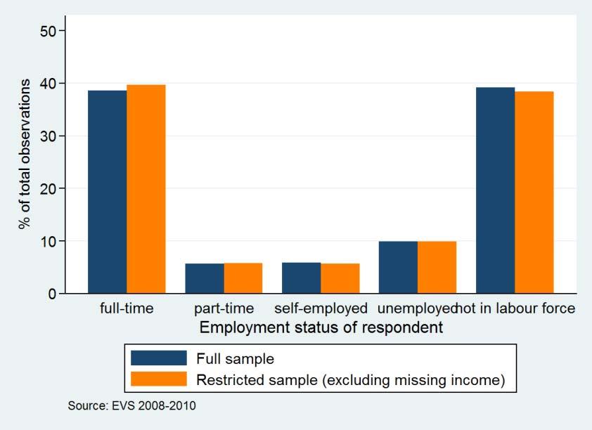
198 Figure C2. Continued. 198

199 health Table C3. Distribution of responses, original categories for select variables. responses (all countries pooled) % of total very poor % poor 4, % fair 15, % good 20, % very good 10, % education inadequately completed elementary education 1, % completed (compulsory) elementary education 4, % incomplete secondary: technical/vocational type/secondary 8, % complete secondary: technical/vocational type/secondary 4, % incomplete secondary: university-preparatory type/secondary 6, % complete secondary: university-preparatory type/full secondary 12, % some university w/o degree/higher education - lower-level tertiary 7, % university w/ degree/higher education - upper-level tertiary 5, % religiousity marital status not al all important 8, % not important 12, % quite important 16, % very important 13, % single/never married 12, % living together as married % married 28, % separated % divorced 3, % widowed 5, % employment status full time 20, % part time 2, % self employed 2, % military service % retired 11, % housewife 4, % student 2, % unemployed 5, % disabled % other % total observations 51,329 Source: EVS

200 Table C4. Summary statistics for select variables, country-specific (all countries). income age children female trust religiousity mean st. dev. mean st. dev. mean st. dev. % % % Albania Azerbaijan Austria Armenia Belgium Bosnia Herzegovina Bulgaria Belarus Croatia Cyprus Northern Cyprus Czech Republic Denmark Estonia Finland France Georgia Germany Greece Hungary Iceland Ireland Italy Latvia Lithuania Luxembourg Malta Moldova Montenegro Netherlands Norway Poland Portugal Romania Russian Federation Serbia Slovak Republic Slovenia Spain Sweden Switzerland Turkey Ukraine Macedonia Great Britain Northern Ireland Kosovo Source: EVS

201 Table C5. Frequency table for self-reported Health, country-specific (all countries). number of responses poor or very poor fair good or very good Albania Azerbaijan Austria Armenia Belgium Bosnia Herzegovina Bulgaria Belarus Croatia Cyprus Northern Cyprus Czech Republic Denmark Estonia Finland France Georgia Germany Greece Hungary Iceland Ireland Italy Latvia Lithuania Luxembourg Malta Moldova Montenegro Netherlands Norway Poland Portugal Romania Russian Federation Serbia Slovak Republic Slovenia Spain Sweden Switzerland Turkey Ukraine Macedonia Great Britain Northern Ireland Kosovo Total 5,690 15,120 30,519 Source: EVS

202 Table C6. Frequency table for Education, country-specific (all countries). number of responses elementary (or less) secondary higher education Albania Azerbaijan Austria Armenia Belgium Bosnia Herzegovina Bulgaria Belarus Croatia Cyprus Northern Cyprus Czech Republic Denmark Estonia Finland France Georgia Germany Greece Hungary Iceland Ireland Italy Latvia Lithuania Luxembourg Malta Moldova Montenegro Netherlands Norway Poland Portugal Romania Russian Federation Serbia Slovak Republic Slovenia Spain Sweden Switzerland Turkey Ukraine Macedonia Great Britain Northern Ireland Kosovo Total 20,990 25,308 5,031 Source: EVS

203 Table C7. Frequency table for Marital Status, country-specific (all countries). single/never married married/living as couple separated/divorced widowed Albania Azerbaijan Austria Armenia Belgium Bosnia Herzegovina Bulgaria Belarus Croatia Cyprus Northern Cyprus Czech Republic Denmark Estonia Finland France Georgia Germany Greece Hungary Iceland Ireland Italy Latvia Lithuania Luxembourg Malta Moldova Montenegro Netherlands Norway Poland Portugal Romania Russian Federation Serbia Slovak Republic Slovenia Spain Sweden Switzerland Turkey Ukraine Macedonia Great Britain Northern Ireland Kosovo Total 12,061 29,446 4,331 5,491 Source: EVS number of responses 203

204 Table C8. Frequency table for Employment Status, country-specific (all countries). number of responses full time part time self employed unemployed not in the labour force Albania Azerbaijan Austria Armenia Belgium Bosnia Herzegovina Bulgaria Belarus Croatia Cyprus Northern Cyprus Czech Republic Denmark Estonia Finland France Georgia Germany Greece Hungary Iceland Ireland Italy Latvia Lithuania Luxembourg Malta Moldova Montenegro Netherlands Norway Poland Portugal Romania Russian Federation Serbia Slovak Republic Slovenia Spain Sweden Switzerland Turkey Ukraine Macedonia Great Britain Northern Ireland Kosovo Total 20,413 2,984 2,957 5,084 19,891 Source: EVS

205 Table C9. Cross-tabulations for categorical variables. health fair poor or very poor good or very good education elementary (or less) 6,597 3,257 11,136 secondary 7,041 2,124 16,143 higher education 1, ,240 marital status single/never married 2, ,094 married 9,045 2,882 17,519 separated/divorced 1, ,335 widowed 2, ,571 employment status full time 5, ,456 part time ,972 self employed ,033 unemployed 1, ,959 not in the labour force 6,821 3,971 9,099 education elementary (or less) secondary higher education marital status single/never married 3,661 7,183 1,217 married 12,181 14,220 3,045 separated/divorced 1,767 2, widowed 3,381 1, employment status full time 5,873 11,602 2,938 part time 979 1, self employed 1,091 1, unemployed 2,345 2, not in the labour force 10,702 8,115 1,074 marital status single/never married married separated/divorced widowed employment status full time 5,375 12,242 2, part time 761 1, self employed 531 2, unemployed 1,791 2, not in the labour force 3,603 10,654 1,247 4,387 Source: EVS

206 Figure C3. Marginal effects at means and average marginal effects with 95% confidence intervals, for income (Ordinal Probit). Figure C4. Marginal effects at means and average marginal effects with 95% confidence intervals, for trust (Ordinal Probit). 206

207 Figure C5. Marginal effects at means and average marginal effects with 95% confidence intervals, for religiousity (Ordinal Probit). Figure C6. Marginal effects at means and average marginal effects with 95% confidence intervals, for bad health (Ordinal Probit). 207

208 Figure C7. Marginal effects at means and average marginal effects with 95% confidence intervals, for good health (Ordinal Probit). Figure C8. Marginal effects at means and average marginal effects with 95% confidence intervals, for marriage (Ordinal Probit). 208

209 Figure C9. Marginal effects at means and average marginal effects with 95% confidence intervals, for separation/divorce (Ordinal Probit). Figure C10. Marginal effects at means and average marginal effects with 95% confidence intervals, for being widowed (Ordinal Probit). 209

210 Figure C11. Marginal effects at means and average marginal effects with 95% confidence intervals, for part-time employment (Ordinal Probit). Figure C12. Marginal effects at means and average marginal effects with 95% confidence intervals, for self-employment (Ordinal Probit). 210