Endogeneity Problems with Binary Treatments: A Comparison of Models

Transcription

1 Endogeneity Problems with Binary Treatments: A Comparison of Models Scott J. Basinger Department of Political Science 447 Philip Guthrie Hoffman Hall University of Houston Houston, TX sjbasinger@uh.edu Michael J. Ensley Department of Political Science 302 Bowman Hall P.O. Box 5190 Kent State University Kent, OH mensley@kent.edu ABSTRACT This article introduces and compares alternative procedures for controlling endogeneity in a regression model with a binary treatment variable. Results are reported from Monte Carlo simulations designed to test the robustness of these procedures under varying levels of endogeneity and instrument strength. The alternative procedures are further compared by replicating an analysis of the influence of presidential appeals on agency appropriations in the United States. Diagnostics for evaluating endogeneity bias and instrument strength are discussed. Practical advice is offered for researchers who are concerned that a binary treatment variable is endogenous.

2 1. Introduction The reality that endogeneity problems pervade the social sciences is both a blessing and a curse. The curse is obvious: uncontrolled endogeneity leads to incorrect estimates of causal effects across widely varying contexts and policies. A prime example is the decades-long debate over the Head Start program s effectiveness, since enrollees may have differed systematically from the population the program sought to aid. The blessing is that endogeneity attracted the attentions of a diverse set of scholars economists, sociologists, political scientists, etc. who generated an equally diverse set of solutions. Unfortunately, each solution is accompanied by its own terminology, notation, and canonical applications. Beyond the syntactical baggage, a technique might be tailored to a particular version of endogeneity, undermining consensus on proper methods. In separate contexts, political scientists adapted methods developed by macroeconomists to resolve simultaneity bias in the presence of reciprocal causation (e.g., Hanushek and Jackson 1977; Jackson 2008), and adapted methods developed by policy-, education-, and laboreconomists to resolve omitted variables bias (e.g., Achen 1986; Bartels 1991). Our focus is on a particularly problematic form of endogeneity problem, treatment selection bias, 1 which is encountered when the potentially endogenous variable is binary. Angrist and Pischke (2009:190) refer ominously to linear models for dummy endogenous variables as forbidden regressions, reflecting the view that the familiar, instrumental-variables practices for dealing with endogeneity must be modified in this context. Thus, the models and diagnostics covered in Jackson s (2008) recent Handbook chapter do not apply directly when the endogeneous variable is not continuous. Goldberger, Heckman, and Maddala, among others, conceived of systems-of-equations solutions to this predicament, which will be the primary focus of this paper. However, the treatment selection bias problem also puts a practitioner into contact with the work of Holland, Rosenbaum, and Rubin, who conceived of matched-sampling solutions. Jackson pronounces, The hope is that these efforts will lead to better tests of causal arguments by avoiding or at least reducing possible endogeneity biases (2008: 428; see also Sekhon 2008). However, 1

3 Ho et al. concede that, from the point of view of the practical researcher, it looks like a cacophony of conflicting techniques, practices, conventions, and rules of thumb (2007: 201). The technical point of this paper, then, is to compare matched-sampling, linear regression, and systems-of-equations methods for studying endogenous treatment effects. In so doing we identify the narrow conditions under which matching methods are sufficient (although not necessarily superior to regression), and we identify conditions under which various methods are to be preferred. The models are engaged in a replication of Canes-Wrone s (2001) analysis of the effect of presidents public appeals. We conclude by offering guidance on choosing between these various approaches, as well as on combining methods for diagnosing whether endogeneity was a problem in the first place. 2. Overt Bias, Ignorability, and Matched Sampling Consider the following analogy. A professor has offered to conduct an optional review session prior to a final examination, but he is uncertain whether the session is a valuable use of students time (not to mention his own time). To evaluate the review session s effectiveness, he asks whether attendance (the treatment, D) improved students scores on the final exam (the outcome, Y). The prima facie causal effect, also known as the observed average treatment effect (OATE), is simply the difference between attendees and absentees mean scores: OATE E(Y D = 1) E(Y D = 0), where E( ) is the expectations operator. Anyone who has experienced an optional review session, either as a student or as an instructor, should be suspicious about the a priori equivalence of the groups of attendees and absentees, due to self-selection. The difference between group averages is likely to produce a biased estimate of the treatment s effectiveness: the bias might be upward if the most intrinsically motivated students are more likely to attend, or downward if students in worst danger of failing are more likely to attend instead. The professor may be misled although it cannot be known in what direction because the study is observational (Rosenbaum 2002) or quasi-experimental (Cook and Campbell 1979), 2

4 defined as: a study intended to assess causal effects of treatments where the rule that governs the assignment of treatments to units is at least partially unknown (Rubin 2006: 7). Suppose that a well-meaning colleague suggests conducting a controlled experiment, by assigning (or encouraging ) a group of students to attend the review session, and denying that opportunity (or encouragement ) to the remaining students. This procedure adheres to the best advice on circumventing selection problems: By creating the treatments of interest [and] by assigning subjects to treatments randomly, the experimenter can be confident (within the limitations established by statistical inference) that any differences observed between subjects assigned to different treatment conditions must be caused by differences in the treatments themselves (Kinder and Palfrey 1993: 11). Unfortunately, forbidding the control group of students from attending the review session may penalize them, akin to denying a treatment to an ill patient. Conversely, requiring the treatment group to attend a review session may harm them by wasting their time or distracting them from other study methods. Lacking the power to exert ex ante control over treatment assignment, the quasi-experimental researcher must confront a basic problem of separating the effect of a treatment from those due to non-comparability between the average units in each treatment group (Cook and Campbell 1979: 6). To draw a valid inference about the causal effect of a treatment, a practitioner might be required to exert ex post control to account for potential biases in treatment selection. The counterfactual model of causality (Morgan and Winship 2007), often known as the Rubin Causal Model, 2 provides a tidy way to distinguish treatment effects from selection effects in quasiexperimental studies. The model is based on the idea that for each subject, one can conjecture two potential or what-if outcomes that might be observed depending on whether the subject is treated. For a subject i, let Y i denote the observed outcome. Let D i denote the observed treatment, such that D i = 1 if she receives treatment (attends the review session), and D i = 0 if she does not. Denote her potential or hypothetical outcomes as Y 1i = (Y i D i = 1) if she is assigned to the treatment group, and Y 0i = (Y i D i = 0) if she is assigned to the control group. Unfortunately, because the analyst makes a single observation for each individual [Y i = (1 D i )(Y 0i ) + (D i )(Y 1i )], individual-level causal effects cannot be calculated a 3

5 predicament that Holland (1986) names the fundamental problem of causal inference. The implication is that one must compute aggregate causal effects, comparing two or more distinct groups. The practitioner might wish to know the average treatment effect on the treated : ATET E(Y 1 D = 1) E(Y 0 D = 1) = E(Y 1 Y 0 D = 1). This quantity is the difference between the average outcome that actually attained for the treated, and the average outcome that would have attained had the identical individuals not received treatment. One cannot estimate this quantity directly, because we observe E(Y 0 D = 0) instead of E(Y 0 D = 1). Therefore, OATE might differ from ATET: E(Y 1 D = 1) E(Y 0 D = 0) = E(Y 1 D = 1) E(Y 0 D = 1) + {E(Y 0 D = 1) E(Y 0 D = 0)} OATE = ATET + {E(Y 0 D = 1) E(Y 0 D = 0)}. The bracketed term in the above equality is treatment selection bias. OATE estimates ATET accurately only if E(Y 0 D = 1) = E(Y 0 D = 0), which requires that the observed average outcome the control group is no different from the hypothetical average outcome that would have attained absent the treatment. Controlled, random assignment s role in experimental design is to ensure that the assignment of the treatment will be independent of the outcome, so that the bracketed term equals zero a priori. If ex ante control through random assignment is unethical or impossible or impractical, 3 or even if the practitioner is concerned with efficiency, then the practitioner might exert ex post control, using background knowledge to achieve conditional independence of the treatment. 4 To illustrate this point, suppose we denote the average treatment effect by τ, the constant by α, and the disturbance term by ε i. Under the assumption of treatment independence, we would initially assume ε i is distributed Normal with zero mean. The observed response will equal: Y i = α + τd i + ε i Conditional expectations for treatment group and control group, respectively, can be written: E(Y i D i = 1) = α + τ + E(ε i D i = 1) E(Y i D i = 0) = α + E(ε i D i = 0) 4

6 The difference estimator (Stock and Watson 2007) equals treatment effect plus selection bias: E(Y i D i = 1) E(Y i D i = 0) = τ + {E(ε i D i = 1) E(ε i D i = 0)}, which is unbiased if and only if disturbances and the treatment are not correlated. Suppose instead that the true model actually equals: Y i = α + βx i + τd i + γ i, where X i is a matrix of covariates perhaps representing aptitude in the class and β is a vector of population coefficients relating aptitude to final exam performance. Assume the disturbances, γ i, are distributed Normally with zero mean. Consequently ε i = βx i + γ i, and the difference estimator yields: E(Y i D i = 1) E(Y i D i = 0) = τ + {E([βX i + γ i ] D i = 1) E([βX i + γ i ] D i = 0)}. By implication, if D i and X i are correlated, then the difference estimator will suffer from omitted variable bias. 5 The prima facie causal effect will over-estimate or under-estimate the true treatment effect depending on whether high-achievers or low-achievers, respectively, are more likely to attend an optional review session. Two approaches to utilizing covariates in order to achieve ex post control are matched-sampling and regression. 6 Matched-sampling models are the counterfactual model s technical counterpart, aiming to mimic controlled experiments by enabling like with like comparisons between treated and untreated subjects. For instance, each treated subject can be paired with a comparison group of the most similar untreated subjects using propensity scores, which are the estimated probability of receiving a treatment; conditional on the covariates; see Rosenbaum and Rubin (1983). The treatment effect is computed as a weighted average of intra-pair differences. The regression model for exerting ex post control is the difference estimator with additional covariates (Stock and Watson 2007): E(Y i X i, D i = 1) E(Y i X i, D i = 0) = τ + {E(γ i D i = 1) E(γ i D i = 0)}, where conditional expectations for treatment group and control group, respectively, could be written: E(Y i D i = 1) = α + βx i + τ + E(γ i D i = 1) E(Y i D i = 0) = α + βx i + E(γ i D i = 0) 5

7 Angrist and Pischke (2009: 80-91) argue that because matching and regression approaches differ only in how they construct weighted averages of the same comparisons between treated and untreated subjects, they will yield similar estimates of treatment effects. Whether these estimates are accurate depends on the conditional independence assumption: conditional on subjects measured characteristics, treatment selection is independent of potential outcomes. If this condition is met, then the treatment selection bias is overt, and can be controlled. Rubin (1978) refers to this situation as ignorable treatment selection, which Barnow, Cain and Goldberger (1981) refer to as selection on observables. 3. Covert Bias and Endogeneity If treatment selection is a function of subjects unmeasured characteristics a situation that Barnow et al. (1981) refer to as selection on unobservables then the conditional independence assumption fails and the treatment selection is unignorable (Rubin 1978). Figure 1 provides two simple illustrations that feature a treatment-selection stage followed by an outcome-determination stage. In Figure 1A, bias is overt, for the variables that systematically determine treatment selection are observed: X denotes a set of observed variables that affect treatment selection and the outcome, and Z denotes a set of observed variables that only affect treatment selection. Idiosyncratic variation in treatment assignment is attributed to one disturbance term, e 1, and idiosyncratic variation in outcomes is attributed to another disturbance term, e 2. In Figure 1B, bias is covert, for a set of unobserved variables, denoted W, systematically affect outcome and treatment selection. 7 Figure 1 about here. Consider again the optional review session analogy. Elements of X are measureable variables that affect students willingness to attend and their likely achievement on the final exam, such as taking the course in their major or performance on a practice test. Elements of W can be conceived of as variables that affect students likely performance and their willingness to attend a review session but are difficult to measure. If X represents the observed aptitude for a course, such as homework scores, then W represents unobserved aptitude, such as test-taking skills. (Students who have a history of testing well may be less 6

8 likely to attend review sessions due to greater confidence in their own abilities.) Z represents factors that affect only the convenience of attending a review session, such as how close to campus a student resides, or whether a student is employed in a part-time, off-campus job. We simulated 1000 observations based on Figure 1B using a latent variable framework. W, X and Z are normally distributed random variables, independently drawn from populations with means 0 and standard deviations 1. Disturbances, e 1 and e 2, are normally distributed random variables, independently drawn from populations with means 0 and standard deviations 1. We generate D* and Y as follows: D i * = ( 1) W i + (1) X i + (1) Z i + e 1i D i = 1 if D i * > 0 D i = 0 if D i * 0 Y i = ( 1) W i + (1) X i + (1) D i + e 2 D* is a latent variable representing students continuously-varying willingness to attend the review session, and D is the observed decision of whether to attend, based on surpassing a threshold (set equal to zero). The true effect of the binary treatment (D) is τ = 1. The observed variables (X) positively affect selection and the outcome, and the unobserved variables (W) negatively affect selection and the outcome. We employ four separate estimators of treatment effect. First, we estimate the naïve observed average treatment effect (OATE) by subtracting the mean Y for absentees from the mean Y for attendees. Second, we use the difference estimator with additional covariates to estimate the treatment effect as the coefficient in an ordinary least squares regression of Y on D and controls. Third, we estimate the average treatment effect on the treated (ATET) using nearest-neighbor propensity-score matching. We estimate a probit regression of D on controls, then use this selection equation s predicted values to pair each treated subject with the most similar untreated subject; differences in the paired outcomes are computed and aggregated by weighted averaging. Fourth, we use a simplistic instrumental variable least squares regression. We estimate a probit regression of D on Z and controls, and then use the predicted probability of D as an instrumental variable in a regression of Y on the controls, excluding Z. 7

9 We estimated the treatment effect four ways under two specifications: W included (in both firstand second-stages) and W omitted (from both stages). If residuals are generated under the assumption that W is unobserved (i.e., u 1i D i * X i Z i and u 2i Y i D i * X i ), they correlate at 0.386; consequently omission of W will lead to an overestimate of the true treatment effect. The 95% confidence intervals for the four methods, for the two specifications, are as follows: W : Included W : Omitted Naïve Difference Estimator [2.511, 2.902] Ordinary Least Squares [0.833, 1.138] [1.771, 2.143] Propensity-Score Matching [0.475, 1.437] [1.860, 2.445] Instrumental Variable Least Squares [0.553, 1.066] [0.269, 1.138] If W is included in the specification, then the bottom three models confidence intervals include the true value of the treatment effect. Ordinary least squares generates the narrowest confidence interval among the three. If we omit W from the specification, then only the instrumental variable model s confidence interval contains the treatment true value (τ = 1); the other three methods overestimate the treatment effects by large amounts. (Appendix Table 1 presents the full estimates from the first- and second-stage models, plus a Heckman-type treatment regression not reported in the text, for both specifications.) This simple simulation provides three insights. First, both propensity score matching and regression suffer from covert bias when treatment selection depends on unobservable and/or unmeasured variables. Because the unobserved characteristic has parallel effect on likely selection and the likely outcome, the prima facie causal effect overestimates the treatment effect. Second, an instrumental variables model can mitigate the bias in the selection-on-unobservables context, as long as an exclusion restriction (Z) can be found. Instrumental variables modeling is just one possible cure to endogeneity problems with a binary treatment; we present more options later in the paper. Third, three estimators generate similar estimates of the treatment effect when D is exogenous (i.e., W included), but generate differing estimates when D is endogenous (i.e., W omitted). This third insight plays a crucial role in how one approaches the task of diagnosing endogeneity, as we discuss in the next section. 8

10 4. Diagnosing Endogeneity Problems How can the practitioner be confident that the analysis is not tainted by endogeneity problems? This difficulty is particularly salient when one must address a concern raised by skeptical or suspicious audiences or readers (e.g., journal peer reviewers). Because OLS generates residuals that automatically are random disturbances, they will be uncorrelated with regressors (any correlation will be subsumed by the estimated coefficients, producing bias) and with the residuals from another equation. Hence, one cannot simply examine the residuals to diagnose endogeneity. The first step in addressing the problem should always be theory, asking: How likely is it that the treatment variable is fixed in repeated samples? Macro-economists treat weather as an exogenous factor, and political scientists treated gender as an exogenous factor (until modern science intervened, that is). If the treatment variable is not fixed in repeated samples, the second step in addressing the problem is to ask: How well do the covariates explain treatment selection? Answering this question requires the practitioner to follow Achen s advice to model both the behavioral outcome of the experiment and the assignment to treatment groups (1986, 37). The difficulty is that there are no clear guidelines on interpreting treatment assignment results. Consider a hypothetical: some scholars have claimed that allowing young children to watch television lessens their attention span. If a first-stage model has extremely strong fit, because measureable demographic factors predispose children both to the treatment (television viewing) and the outcome (attention span), then the causal claim most likely would be undermined if the selection effect was controlled. But, a first-stage model might have extremely poor fit for two, opposite reasons: because the primary determinants of assignment are unobserved factors, such as parental attitudes or care-giving tendencies, or because television viewing is an unpredictable phenomenon, and can be treated as if it is randomly assigned. Simply examining propensities to view television does not offer a true escape from the predicament. Addressing the problem requires using the results of the selection model as a mechanism for forming comparisons between estimators. For instance, matched-sampling estimators prove their worth by showing covariate imbalance before and after matching. Analogously, instrumental variables 9

11 estimators, which assume a treatment is endogenous and attempt to confront the endogeneity directly, can prove their worth through a comparison to a baseline estimator that assumes a treatment is exogenous. The simplest version of this comparison has three elements. The researcher estimates an OLS model, which is consistent if the null hypothesis of endogeneity is true, and further, is guaranteed to be efficient whether the null hypothesis of exogenity is true or false (Maddala 1983). The researcher also estimates an instrumental variable model, which is consistent if the null hypothesis of exogeneity is false. Third, one assesses whether the vector of estimated coefficients differs by more than just sampling error; the test statistic is distributed χ 2 with one degree of freedom for each endogenous regressor (see Hausman 1978). 8 In short, diagnosing endogeneity with binary treatment effects requires both thoughtfulness about endogeneity s potential sources and willingness to estimate multiple models, compare results, and discard findings that are tainted by endogeneity bias. In the next section we turn to a more detailed presentation of a broader set of options available to the researcher. 5. A Menu of Solutions In an ideal world, regressors and the disturbance term are uncorrelated, and OLS or matching produces unbiased estimates of treatment effects. When this assumption fails, the practitioner needs to be aware of the other options. We offer five solutions, three of which utilize instrumental variables, and the remaining two utilize control function approach due to Heckman (see Barnow et al. 1981; Heckman and Robb 1985). Instrumental variables (IV) methods for binary endogenous regressors are adapted from the twostage least squares (2SLS) model the solution offered by economists since the Cowles Commission. The basic idea is to find a source of autonomous variation (see Aldrich 1989); incorporating this variation can purge regressors of their correlation with the disturbance term. If the endogenous variable is continuous, then the first stage would be a regression of the endogenous variable on a set of exogenous variables, including purging variables that (are conjectured to) affect the treatment but not the outcome. The second stage would be a regression of the outcome variable on the exogenous variables, minus the 10

12 purging variables, plus the predicted values from the first-stage regression as substitute for the original values of the endogenous variable. Assuming that the instruments are valid, this process produces consistent estimates. But if a possibly endogenous treatment variable is binary, this complicates the process of creating an instrument, for the same reasons that a binary dependent variable complicates regression analysis (see Aldrich and Nelson 1984). The first IV approach to consider, one that requires the smallest modification to 2SLS, uses a linear probability model (LPM) to estimate the first stage equation, using Goldberger s (1964) corrections to standard errors. The predicted probabilities calculated from the first stage are then used in the second stage, after resetting any out-of-bounds estimates. Achen (1986: 44-45) refers to this process as generalized two-stage least squares (G2SLS). Achen uses this method to show that pretrial detention actually has no effect on increasing the probability of a conviction, once the analyst properly controls for the nonrandom assignment of arrested individuals to detention or release (see Schneider et al. (1997) for another application). Proponents of this model contend that because the first-stage equation is a linear model, coefficients in the selection equation can be interpreted straightforwardly as changing the probability of treatment. A second IV model uses nonlinear regression for the first stage equation. Achen (1986: 46-48) describes a handful of nonlinear methods, such as including squared and cubed terms, but the model that has most in common with propensity score matching and other methods we discuss below uses probit to estimate the treatment selection coefficients. This is one version of what Alvarez and Glasgow (1999) label two-stage probit least squares (2SPLS). 9 The predicted values from the first-stage probit model can be substituted for the actual values of the treatment variable in the second-stage least squares model. Angrist and Pischke (2009: 190-1) warn against using this method, for if the first-stage is not probit (i.e., if disturbances in the treatment-selection stage are not distributed Normal), then there is no guarantee that first-stage residuals will be uncorrelated with fitted values of the endogenous treatment and covariates. A third IV model, proposed by Wooldridge (2002: ) and endorsed by Angrist and Pischke (2009: 191), inserts an intermediate stage, and hence we refer to the procedure as the three-step approach. 11

13 Step 1 is a probit regression of the endogenous dummy variable on the exogenous variables and the exclusion restrictions. Step 2 is a least squares regression of the endogenous treatment variable on the exogenous variables and the predicted probabilities from Step 1. Step 3 is a least squares regression of the outcome variable on the exogenous variables and the predicted values from Step 2. The procedure begins no differently from the probit model of selection, and hence exclusion restrictions must be found. The second step uses first-step predicted probabilities as its exclusion restrictions; the intermediate step allows the researcher to employ a non-linear probability for the assignment of the treatment but does not impose a specific distributional assumption for the probability model. A salient concern with all IV methods is that the system of equations must be identified in order to obtain estimates of the parameters. Since many explanatory variables appear in both the selection and outcome equations, there can be a high degree of multicollinearity between the instrumental variable and the covariates. These IV procedures may be technically identified even if both equations employ the same variables, since the predicted values from the selection equation enter the outcome equation in a nonlinear form. 10 Exclusion restrictions, or purging variables, are notoriously difficult to find, since they must be exogenous, meaning that they do not affect the outcome, and relevant, meaning that they do affect treatment selection. If the exclusion restrictions weakly influence selection, IV methods can be badly inconsistent even in large samples (Bound, Jaeger, and Baker 1995). If the exclusion restrictions do indeed affect the outcome, i.e., are quasi-instruments, then instrumental variables methods may be plagued by excessive mean-squared errors (Bartels 1991). In either situation, i.e., weak instruments or quasi-instruments, the practitioner might do better to ignore the endogeneity problem and employ OLS. We discuss tools for diagnosing instrument validity in the conclusion. Two alternatives that do not employ instrumental variables are control function (CF) models based on the work of Heckman (1978, 1979, 1990, 2000). 11 The Heckman models can be estimated via a two-step approach or by Full-Information Maximum Likelihood (FIML) methods; the latter has efficiency advantages in the presence of selectivity bias (Hartman 1991), but is theoretically less robust with respect to specification errors because it assumes bivariate normality of the errors (Alvarez and Glasgow 1999). 12

14 Heckman s idea is to estimate a model of the treatment assignment, and then use the predicted probability of treatment as a separate covariate, called a control function or a hazard function. Let us illustrate this approach using the two-stage method, in which the first stage is a probit model of treatment selection, using the familiar latent variable formulation: D i * = Z i α + u i D i = 1 if D i * > 0 D i = 0 if D i * < 0, where Z is a vector of exogenous characteristics that influence whether the observational unit receives the treatment, α is a vector of coefficients to be estimated, and D* is a continuous, latent variable for the binary, observed treatment variable D. Further, let Y denote the outcome of interest, let X denote a vector of variables that explain the outcome according to the coefficients β: Y i = X i β + τd i + γ i. The error terms from the selection equation (u i ) and outcome equation (γ i ) can be correlated. If we assume errors are generated from a bivariate Normal distribution, then we can derive the following regression equation for treated subjects (see Greene 2003, ): E[Y i D i =1, X i ] = X i β + τ + E[γ i D i =1] = X i β + τ + ρσ e [ ], where φ denotes the standard normal density function, Φ denotes the standard cumulative normal distribution function, ρ is the correlation between the disturbances in the selection and outcome equations, and σ e is the standard deviation of the errors in the outcome equation. We can also derive the regression equation for untreated subjects: E[Y i D i =0, X i ] = X i β + E[γ i D i =0] = X i β + ρσ e [ ]. The treatment effect is defined as the following difference: 13

15 E[Y i D i =1, X i ] E[Y i D i =0, X i ] = τ + ρσ e [ ], where φ i =φ(z i α) and Φ i =Φ(Z i α). The consequence of using OLS to estimate the treatment effect is indicated by the value of the second term on the right-hand-side of this equation. The OLS estimate of τ will be unbiased only if ρ = 0. Because σ e and are always positive, the sign of ρ indicates the direction of the bias. If ρ > 0 then ordinary least squares will overestimate the treatment effect; if ρ < 0 then regression will underestimate the treatment effect. Heckman s solution is to incorporate information about treatment selection into the outcome equation by adding a regressor, a selectivity-correction variable,, defined as follows: if D i =1, if D i =0. If we assume that the joint distribution of the error terms in the selection and outcome equation is bivariate normal, estimates of α can be obtained from a probit model estimated via a maximum-likelihood procedure, 12 and estimated values of λ can be calculated and included in the second-stage OLS regression. The Heckman FIML model provides a direct test for endogeneity through a test of the significance of. The Heckman two-step procedure provides an indirect test for endogeneity, estimating s statistical significance through the estimated coefficient on the selectivity-correction variable (,). In fact, all five techniques that we have discussed provide a method for testing for endogeneity of the treatment. For the three IV models, one can use the (Durbin-Wu-) Hausman test for endogeneity described in Section 4. If a researcher chooses to confront the endogenous treatment selection problem, then immediately after estimating any of these models, the next step should be assessing evidence of endogeneity, since OLS is more efficient if the treatment is (conditionally) exogenous. With numerous options available for confronting endogeneity problems, it worth assessing how these procedures perform under different conditions. In the next section we report on simulations that 14

16 investigate the estimators performance under varying levels of endogeneity, varying levels of instrument strength, and varying distributions of the errors in the first-stage treatment equations. 6. Monte Carlo Simulations In order to examine the properties of these estimation procedures, we performed Monte Carlo simulations. The sample size for each simulation is 1000 observations. We created 28 separate conditions from varying the distribution of the disturbance term in the treatment-selection equation, the degree of endogeneity (i.e., correlation between the disturbances in the two equations), and the strength of the instruments. For each of the 28 conditions, we repeated the simulation 1000 times. After every simulation we computed an estimate of the treatment effect using ordinary least squares and each of the five estimation procedures discussed in Section 4. The underlying model is as follows: d* = α z + 0.5x + e 1 d = 1 if d* > 0 d = 0 if d* < 0 y = 1d + 1x + e 2 The treatment effect is τ = 1, as seen in the outcome equation. The parameter α in the treatment-selection equation determines the relevance of the instrument, i.e. the strength of the relationship between the instrument and the endogenous variable. Each equation has an associated disturbance: e 1 is the error term for the treatment equation and e 2 is error term for the outcome equation. The error terms are generated in the following manner: e 1 = F(0,1) e 2 = N(0,1) + δe 1 where F( ) is a generic probability distribution and N( ) is the Normal distribution. To compare the different procedures and to examine their robustness, we utilize three different functional forms for F( ). First, we generated treatment-selection disturbances using a Normal distribution. The Heckman FIML model, the Heckman Two-Step model, and the 2SPLS model all employ a probit model in the first stage, 15

17 therefore the normality assumption favors these models. However, incorrect distributional assumptions might have disastrous effects, particularly for the FIML model. Therefore, we generated treatmentequation errors using the logistic distribution, which is symmetrical and bell-shaped like the Normal distribution, but with fatter tails. We chose the logistic distribution since it is similar but not identical to the Normal distribution, and thus represents a small departure from normality. Following Vella and Verbeek (1999), who investigate models with endogenous treatments effects, we also generated first-stage errors using a uniform distribution, which represents a large departure from Normality. Regarding the degree of endogeneity, we generate e 2 as a weighted combination of e 1 and a standard Normal random variable. We chose seven distinct values for the weight, δ, to produce seven different levels of endogeneity, producing correlations between the two equations errors (denoted ρ e1,e2 ) that range from 0.0 to The error terms were standardized to have a mean of 0 and a variance of 1 before parameter estimations were carried out. As we discussed above, invalid instruments can undermine the value of performing IV analysis, particularly because instruments that are truly autonomous may be only weakly related to the treatment selection. To examine the properties of the estimators under varying levels of instrument relevance, we performed simulations using both strong- and weak-instrument conditions. 13 In rare instances, the FIML model failed to converge in the Monte Carlo simulations using the default optimization algorithms. Generally speaking, this is more likely to occur when the degree of endogeneity is high (i.e. the error correlation is 0.9 or greater), when the instrument is weak, and when the sample size is small. 14 We minimized this problem s occurrence by holding the sample size at 1000, but closed-form solutions for the first and second derivatives of the log-likelihood function do not exist for the Heckman FIML procedure. In such a situation, when convergence is not assured, the researcher has a choice of updating algorithms that are asymptotically equivalent. Following Eliason (1993), we set the optimization sequence to 50 iterations under the Broyden, Fletcher, Goldfarb, and Shannon (BFGS) algorithm to get close to the solution, then switch to 5 iterations under the Berndt, Hall, Hall, and 16

18 Hausman (BHHH) algorithm, which is more efficient. This sequence was repeated until convergence was achieved, which happened in less than 500 iterations in every one of the simulations reported below. To compare the properties and performance of each procedure, and to evaluate the consequence of changing levels of endogeneity and instrument relevance, we report and analyze three criteria: average bias, mean-squared error, and coverage. The bias of an estimate is the difference between the true value of the treatment effect (τ = 1) and the estimated treatment effect. In Table 1 we report the average bias in treatment effect estimates, across 1000 simulations for each condition. As a baseline, consider the average bias of ordinary least squares (shaded rows), noting that the distribution of the treatment-selection stage error term is irrelevant for the OLS procedure, since treatment-selection is not part of the estimation procedure. OLS is, on average, barely biased when there is no endogeneity problem (ρ e1,e2 = 0). As the level of endogeneity increases (ρ e1,e2 increases moving across the columns, from left to right), OLS becomes more biased. To interpret the bias figures, observe that when the disturbances are correlated at 0.1, the average bias is between and , indicating that the average estimated treatment effect is 15% to 17% larger than the true treatment effect. When the correlation reaches 0.7, the average bias is over 100% of the true value for any of the three functional forms (Normal, logistic, or uniform). INSERT TABLE 1 How do the other estimators perform? As long as the errors are drawn from a Normal distribution and the instrument is strong, the average bias never exceeds 2% for the Heckman Two-Step model, 2SPLS, Three-Step, or Heckman-FIML. Average bias of the LPM model is higher, but still never exceeds 10% of the true treatment value. When we compare the results for strong and weak instruments maintaining the assumption of Normal errors we observe that average bias is consistently greater for the three IV models than for the two CF models. The Heckman Two-step method performs well across the board, consistently yielding less average bias than the IV models. The Heckman-FIML model performs poorly for medium levels of endogeneity, but performs excellently for both high and low levels of 17

19 endogeneity. The 2SPLS models performing slightly better than the Three-Step model in the weak instrument condition, and the LPM performs consistently worst, as usual. The average biases of the estimates drift further apart once the true data generating process deviates from Normality. When errors are generated from a Logistic distribution, the average bias for the Three-Step method or the 2SPLS model is always lowest. In fact, a comparison of the results for the Normal and Logistic functional forms reveals little change in the Three-Step method s average bias under different, indicating its superior robustness. The two CF approaches yield more biased estimates than the Three-Step model and 2SPLS, especially at higher levels of endogeneity (higher values of ρ e1,e2 ). The average bias in the Heckman Two-step estimates is small, about 3 percent of the true value of the treatment effect if the correlation between the errors is large. The average bias of the Heckman-FIML estimates is roughly three times as large as the Two-Step model s bias when errors are generated with a logistic functional form. The dangers of imposing the wrong distributional assumption become most evident when we examine the bias with uniform distributed errors. Although the average bias worsens for all methods, the Heckman Two-Step model yields less biased estimates than the Heckman-FIML model. To summarize the discussion of bias, we find first that the level of endogeneity has barely an effect on the two non-linear IV models (2SPLS and Three-Step) and on the two CF models when the errors are drawn from a Normal functional form and the instrument is strong. When the instrument is weak, the Heckman Two-Step model is less biased than the two non-linear IV models, and its superiority becomes more apparent as the level of endogeneity grows. However, the distribution used to generate the errors interacts with the level of endogeneity, generating substantially greater bias when the errors are generated from distributions with thicker tails (Logistic or uniform). The Heckman-FIML model s bias increases most dramatically with increasing endogeneity if the Normality assumption is violated. A second criterion for judging among estimators is the mean-squared error (MSE), which is the sum of the squared differences between the estimated and true treatment effect. MSE also equals the sum of variance and squared bias, so the least biased estimators are expected to perform better on this criterion as well. We present the average mean-squared error for the different conditions in Table 2. As the 18

20 baseline for comparison, the OLS simulation results show that as the correlation between the error terms increases, the MSE far exceeds the other approaches. If the expected correlation is very low (i.e., less than or equal to 0.1) and/or the instruments might lack validity, then OLS may be advisable, as Bartels (1991) has suggested. However, if we are suspicious of endogeneity but confident in the instruments, then almost any method for controlling endogeneity is an improvement over OLS. The MSE results indicate that the Heckman FIML model yields a lower MSE than any alternative approach if the first stage errors are drawn from a Normal or Logistic distribution. Under the Normal functional form, this was to be expected, given that maximum likelihood estimation is efficient and consistent, and it is reassuring that the Heckman-FIML model s MSE is still lowest when the true data-generating process follows the Logistic model. If the true data-generating process is Uniform, the MSE of the Heckman Two-Step approach is lowest if the correlation is 0.9 or greater. The Heckman Two-Step method and the other three nonlinear models yield similar MSE values to each other regardless of the correlation between the errors. Based on a MSE criterion, the FIML approach appears superior (except when the level of endogeneity is low, when OLS may be the preferred approach); the superiority is even greater for the weak instrument and Logistic-distributed errors conditions than with Normal errors and strong instruments. 15 INSERT TABLE 2 A third criterion for choosing among estimators is the coverage rate, defined as the percent of simulations for which the true value located in the estimated 95% confidence interval. We present the coverage rates for each of the six estimation procedures in Table 3. Naturally, we expect that the true value of the treatment effect should fall in the estimated confidence interval 95% of the time. For OLS, we see that the coverage rate is close to 95% when there is no endogeneity problem, but quickly falls as endogeneity rises. When the correlation between the disturbance terms is 0.3 or greater, the coverage rate for OLS is 0% for the 15,000 simulated samples. Under the assumption of normality, we find that the coverage rate is close to 95% for the other methods. The coverage rate for the LPM approach is consistently greater than 95% regardless of the level of endogeneity or distributional assumption. How can it be that the model with the worst bias has the best coverage? The simple answer is that the 19

21 confidence interval generated by the LPM is too large. The Heckman FIML approach looks slightly less appealing under Normal errors, and its coverage rate decreases as the level of endogeneity increases for the logistic or uniform distributions. The other methods are more promising, in particular the Heckman Two-Step model and the Three-step model. The 2SPLS model yields coverage rates that are consistently too high, while coverage rates for the Heckman Two-Step model and the Three-step model are consistently close to 95%, for all levels of endogeneity and distributional assumptions. INSERT TABLE 3 In the final section of the paper we offer guidance on which method or methods would be best depending on the circumstances the researcher confronts. Based on the evidence on bias, mean-squared error, and coverage, the simulations guide us to endorse the Heckman Two-Step or the Three-Step IV model, assuming the researcher faces an endogeneity problem. These procedures have consistently low MSE and appropriate coverage rates. The Heckman Two-Step procedure generates slightly more biased estimates if errors at the treatment-selection phase do not follow a Normal distribution, but is more robust to weak instruments than the IV approaches. The Three-Step IV approach has several notable advantages, particularly robustness to misspecification, and the ease with which it can be extended to multiple endogenous variables, some of which may be continuous and some of which may be dichotomous. The Heckman FIML procedure is least biased and has lowest MSE when the true data generating process is Normal, but we hesitate to recommend it because of its sensitivity to misspecification. When the errors are generated from a non-normal process, the Heckman-FIML approach yields biased estimates and a low coverage rate, especially as endogeneity increases. 7. Application to Presidential Leadership in Congress To demonstrate the consequences of using these different procedures, we replicate the analysis of Canes-Wrone (2001) who examines whether presidents going public impacts success in Congress. 16 Canes-Wrone measures success by calculating the proportional difference between a president s requested appropriation and Congress s actual appropriation for various government agencies. Dividing the raw dollar amounts by the agency s budget from the previous fiscal year ensures that success is 20

22 comparable across agencies of various sizes. Canes-Wrone theorizes that the binary treatment, a public appeal by the president, is endogenous to success because presidents are strategic in selecting which agencies to emphasize. Presidents will not wish to be perceived as foolishly wasting their political capital on an unpopular proposal, or on a proposal that is already likely to pass. If a president is more apt to make a public appeal when it is likely to bend Congress to the president s will, then factors affecting success will also affect appeals. A practical reason for replicating this analysis is that Canes-Wrone (2001) provides an instrument that passes both tests of validity: the size of the agency, measured by the previous year s budget. First, with regard to instrument strength, presidents are more likely to allocate their scare time to larger and hence more salient agencies, all else being equal. In the results reported in Table A2, the coefficient for agency size is statistically significant (p < 0.05) in every specification except in the LPM (where p = 0.07). 17 Second, with regard to instrument exogeneity, notice that the dependent variable is the proportional change in the request, which is, by construction, unaffected by agency size. An added practical reason to replicate Canes-Wrone s (2001) research is that the analysis utilizes more than 1000 observations, providing a large enough sample to estimate the various procedures discussed in this paper. 18 It is important to note that Canes-Wrone (2001) estimates a simultaneous equation model with two jointly endogenous variables: public appeals and presidential budgetary success. 19 Simultaneous estimation of these two equations may be more efficient, but two equations can be estimated separately without compromising consistency. Given our interest in models for estimating a dichotomous treatment variable s effect on a continuous response variable, we restrict our attention to the budgetary success equation. The dependent variable is the negative absolute value of the difference between the president s requested appropriation and Congress s final appropriation; these figures are normalized by dividing by the previous year s appropriation. The treatment of interest is a public appeal, measured using a dummy variable coded equal to one if the president made a statement about the agency s budget in a nationally televised address, and coded equal to zero otherwise. Numerous control variables are specified in the 21

23 model; we present the full models in the appendix and urge the reader to consult Canes-Wrone (2001) regarding justification and coding conventions for the control variables. Canes-Wrone predicts and finds a positive treatment effect: a presidential appeal leads to greater presidential success (Table 2; 2001: 325). We wonder, does the estimated treatment effect vary across estimation procedures? Table 4 presents the estimated treatment effects, along with estimated standard errors and p-values, for least squares regression and matched-sampling (which assume conditional exogeneity) and the five alternative methods (which assume endogeneity). The point estimate and 95% confidence interval estimates are also displayed in Figure 2. Table 4 also reports the appropriate p-value from a test of whether the treatment variable is actually endogenous. For the Heckman-FIML model, the proper endogeneity test is a likelihood ratio test of the two equations independence, with ρ = 0 being the null hypothesis. For the Heckman Two-Step model, the proper endogeneity test is a test of the hypothesis that the control function coefficient (λ) equals zero. For the IV models, the proper test of endogeneity is a Hausman test. In all cases, the null hypothesis is that the treatment variable is exogenous. The first two rows of Table 4 present treatment effect estimates using Ordinary Least Squares and Nearest-Neighbor matching (nearest k-neighbor matching with bootstrapped standard errors, where k=3). The OLS estimated coefficient is positive, consistent with Canes-Wrone s theory, but the magnitude of the coefficient is small (β = 0.057) relative to the standard deviation of the dependent variable (0.190). Matching produces a slightly larger estimate of the treatment effect (β = 0.066). Both estimated treatment effects are statistically significant at conventional levels. The other five methods produce larger estimates of the treatment effect than the OLS or matching methods. The Heckman-FIML procedure produces an estimate of the treatment effect that is only slightly larger (β = 0.082) and this coefficient is significantly different from zero, however the likelihood ratio test of endogeneity fails to reach the conventional level of statistical significance (p = 0.47). The Heckman- FIML results thus suggest that controlling for endogeneity is not necessary and the OLS estimates are valid. As we have discussed, however, FIML models lack robustness if the model is mis-specified. To use 22

24 the Heckman model appropriately, it must be the case that arrows between the outcome variable, presidential success, and the treatment variable, presidential appeals, do not run in both directions. Canes- Wrone (2001) theorizes that causality is reciprocal, and if she is correct, then the FIML estimates must be invalid. This critique only applies to the FIML estimates, because the models utilizing two or more steps (i.e., Heckman two-step, 2SPLS, Wooldridge s three-step method, and linear probability models) do not require that causality is unidirectional. The Heckman Two-step estimate of the treatment effect is quite large (β = 0.234) relative to the OLS and Heckman-FIML estimates, and it is statistically significant (p = 0.03). The test for endogeneity falls in a grey area regarding statistical significance (p = 0.09). The 2SPLS model and the Three-Step model also produce estimates of the treatment effect that are similar in magnitude, more than three times as large as the OLS and matching estimates, but they fall short of conventional levels of statistical significance (p = 0.11), and the endogeneity tests for these models are insignificant (p = 0.21). Finally the Linear Probability Model produces an estimate that of the treatment effect that is far larger than any of the other models (β = 1.093) and that approaches conventional levels of statistical significance (p = 0.08). Most likely, this large coefficient results from fitting a linear model to a rare event process. Out of 1,124 observations, the president made a public appeal only 88 times, which amounts to a probability of a public appeal below 7 percent. In addition to providing the largest estimated treatment effect, the LPM procedure also provides the most statistically significant test statistic suggesting that endogeneity is a problem; the Wu-Hausman test s p-value is less than But given the availability of other suitable methods, discussed herein, and given the results from the Monte Carlo simulations, the use of a LPM model with dichotomous treatment variable is hard to justify. Our aim in replicating this analysis was not to question Canes-Wrone s findings, but rather to utilize available data to demonstrate that treatment effects estimates are sensitive to the chosen method. The results are consistent in finding that presidential appeals have a positive effect on presidential success, as hypothesized, and most effects are larger than Canes-Wrone estimated

25 8. Discussion Given the prevalence of observational, non-experimental data in social science, researchers must be constantly wary of endogeneity problems, which can result from omitted variables, measurement error in independent variables, reciprocal relationships, and non-random treatment assignment. While methods for confronting endogeneity have proliferated, an understanding of which methods are appropriate under which conditions remains elusive. In this article, we have surveyed methods for confronting endogeneity bias in a specific yet common case, when the potentially endogenous treatment is a dichotomous variable and the outcome of interest is continuous. Based on the results of Monte Carlo simulations and a test of presidential going public, we offer some practical advice for researchers who suspect that they may have an endogenous binary treatment variable. We suggest a practitioner follow a seven-step process. 1. Pause, and consider sources of a possible endogeneity problem The first step should be to push back from the keyboard and consider carefully the source or sources of suspected endogeneity. (Fortunately, journal peer reviewers and brownbag audiences often are willing, or even delighted, to share their suggestions about probable sources of endogeneity.) If the endogeneity problem originates in non-random assignment of a binary treatment, then the practitioner should first consider if assignment is based on observable or unobservable factors. If the latter, then an IV or CF approach might be worth considering although not necessarily worth adopting unless other conditions are satisfied. The next steps require the researcher to estimate multiple models, and utilize the results of multiple estimations to identify the proper model. 2. Estimate ordinary least squares regression 3. Estimate instrumental variables regression 4. Perform a Hausman test of endogeneity 5. Perform a test of instrument strength Ordinary least squares estimation of a system of equations is guaranteed to be efficient regardless, and consistent under the null hypothesis of exogeneity (Maddala 1983). An instrumental variable model will be inefficient, but will be consistent under the alternative hypothesis of endogeneity. In our opinion, 24

26 the researcher should estimate two models: OLS and Wooldridge s (2002) Three-Step IV model. Comparing the estimated coefficients on the treatment variable from the OLS and IV models is worthwhile and we show such a comparison in Figure 2 but it is only a heuristic device. The fourth step should be an examination of the estimated coefficients; if the null hypothesis of exogeneity is correct, then the two vectors of coefficients should differ only by sampling error. The Hausman test, described earlier, provides a straightforward method for testing the null hypothesis of exogeneity; rejection of the null hypothesis indicates that OLS is inconsistent. However, this result would not imply that an OLS estimate of the treatment effect is inferior to an IV estimate, for an IV model is only as good as its exclusion restrictions. Instrument strength can be assessed a variety of ways in a canonical 2SLS model, but options are limited with a binary endogenous variable. Two options for assessing instrument strength are the statistical significance of the purging variables in the first-stage model and the LR test statistic from the joint hypothesis test of excluding the purging variables from the first-stage probit equation. If the null hypothesis of instrument irrelevance is rejected, and if the Hausman test rejected the null hypothesis of exogeneity, then the IV estimates earn more confidence. 6. Estimate control function regression 7. Perform a Hausman test of endogeneity In our Monte Carlos simulations, the CF procedures were most robust to weak instruments. This alone makes the two-step Heckman procedure worth considering. Therefore, regardless of instrument strength because instruments that are too strong might be quasi-instruments the sixth step is to utilize a CF model, and in particular, Heckman s two-step model, to estimate the treatment effect. The seventh step is another test of endogeneity, examining the statistical significance of the selectivity-correction variable and/or the statistical significance of the estimated ρ. In our replication of Canes-Wrone s analysis, the Three-Step IV model and the Heckman Two-Step model produced nearly equal estimates of the treatment effect, and nearly equal p-values in the tests of endogeneity. We would report all three estimates, which agree that presidential leadership in Congress is effective. Reporting at least OLS and one other estimate would indicate to the reader the size and direction of possible endogeneity bias. 25

27 As for the opposite question, of what a practitioner should not do, notice that we have not endorsed three of the five models. A FIML model, in which the two-equation model is estimated simultaneously, is sensitive to misspecification. Given that social scientists often must use available data, specification issues present a constant risk, including the difficulties of finding good instruments and measuring concepts. It is concerning to note that FIML estimation is the default in STATA for both the Heckman treatment-selection (treatreg) and sample-selection models (heckman and heckprob). Although the Heckman FIML model has an efficiency advantage vis-à-vis the multi-step models, our Monte Carlo simulations indicate that the FIML version is the least biased under a slim set of circumstances. We also have not endorsed use of an LPM model or the 2SPLS model. Among the IV procedures, the main advantages of the LPM were two: researchers familiarity with linear regression, and the ease of interpreting first-stage coefficients. As political scientists comfort level with probit and logit models have grown, however, and as statistical packages have evolved, these advantages have been negated. More importantly, the LPM procedure performed poorly relative to the other two-step methods, producing greater average bias and overly optimistic coverage rates. More generally, we should re-emphasize that these methods rely on the use of instruments that are strong and autonomous. Other scholars have addressed the issue of the reliability of instruments in the two-stage least squares model with two continuous variables (Bartels 1991; Bound et al 1995). The advice offered in that set of circumstances applies here as well: if the instruments are too weakly related to the treatment, or if the instruments are too strongly related to the outcome, then a model that ignores the endogeneity may be preferred on a MSE criterion, since the standard errors are larger in the two-step procedures without any significant reduction in bias. Unfortunately, there is no real substitute for locating and using valid instruments. So we recommend, finally, that any scholar who draws interpretation from an IV model provide a robust theoretical justification for the validity of the instrument, should consider trying different instruments or combinations of instruments (if available), and should utilize multiple methods to validate the estimates of any individual model. 26

28 9. Endnotes 1 Cox (1988) refers to this as the problem of non-random assignment, as distinct from non-random selection (which we would refer to as sample selection bias ). In both situations, the core problem is unobserved data. With non-random selection, no measure of the outcome variable is observed for units who are not in the sample. With non-random assignment, an outcome is observed for all units, but not in both the treated and the untreated states. Bias can result if the treated and untreated units, or if the sampled and unsampled units, differ systematically. See Achen (1986), Dubin and Rivers (1989), and Sigelman and Zeng (1999) on sample selection bias. 2 Although primarily associated with Rubin (1974, 2006), Holland s (1986) and Rosenbaum s (2002) contributions should not be underestimated. Rubin also gives a great deal of credit to Cochrane. Brady (2008) and Cortina (2009) provide recent and easily digestible introductions. 3 The bracketed term rarely equals zero a posteriori. Quoting Morgan and Winship (2007: 40): For randomized experiments, the treatment variable is forced by design to be independent of the potential outcome variables. However, for any single experiment with a finite set of subjects, the values of d i will be related to the values of y i1 and y i0 because of chance variability. 4 See Manski s (1993: 24) definition of a treatment effect: the change in average outcome if one were to replace a hypothetical situation in which a person with attributes X were exogenously assigned to treatment 0 with another hypothetical situation in which a person with attributes X were exogenously assigned to treatment 1. 5 Stock and Watson urge testing for random receipt of treatment by regressing treatment dummy on covariates, and computing the F-statistic to test whether coefficients are zero. If the treatment is randomly received, then including covariates still would reduce inefficiency (see Angrist and Pischke 2009). 6 Morgan and Winship (2007) present a matching-heavy approach that is critical of regression, and Angrist and Pischke (2009) present a regression-heavy approach that is critical of matched-sampling. We recommend that the interested reader consult both for balance. 27

29 7 If variables in W affect treatment selection but not the outcome, then they would be classified among e 1 ; if variables in W affect the outcome but not treatment selection, then they would be classified among e 2. 8 Obviously, we are aware that Stata performs this as a post-estimation command estat endog, following ivregress, or as ivendog, following ivreg2 (Baum, Schaffer and Stillman 2003). 9 Alvarez and Glasgow emphasize 2SPLS in a situation when the endogeneous regressor is continuous and the outcome variable is dichotomous. We refer to this situation as a dosage selection bias problem rather than treatment selection bias, although some readers might view the difference as semantic. 10 Vella (1998, p. 135) endorses the use of exclusion restrictions, because although the predicted values from the probit model are nonlinear, it is linear in some ranges. Based on the work of Leung and Yu (1996), Vella notes that if there is sufficient variation in some the exogenous variables, then exclusion restrictions may be not be necessary for identification. However, without valid exclusion restrictions, these results should be treated cautiously (see Sartori (2003) for the same point in a different context). 11 Heckman s motivation was to unite classical Cowles Commission simultaneous equations theory and models of discrete choice originating in mathematical psychology in order to produce an economically motivated, low dimensional, simultaneous equations model with both discrete and continuous endogenous variables (2000: 267). Barnow et al. (1981) deserve credit for the application of Heckman s models to treatment selection problems; they also cite Amemiya (1978) and Maddala and Lee (1976) prominently. 12 Although economists and statisticians have investigated semi-parametric and non-parametric models of self selectivity, which do not rely on particular distributional assumptions, the more familiar parametric solutions to self selectivity do remarkably well; see Angrist (2001); Heckman (1990); Manski (1993). 13 In the strong-instrument condition, we set α.4306, to achieve a correlation of 0.3 between the instrument (z) and the latent variable (d*). In the weak-instrument condition, we set α.1266, to achieve a correlation of 0.1 between z and d*. Weakening the instrument has direct effects on the properties of the estimators, however we found no interesting interactions between instrument strength and first-stage equation error term functional forms. Hence, we report simulation results for the logistic and uniform 28

30 distributions only for the strong instrument condition. 14 In a set of simulations with a smaller sample size (N=200) that are not reported in this paper, there were a few instances (approximately 1 in every 1000) in which the FIML model failed to converge. 15 These results parallel Hartman s (1991) findings for the Heckman selection model. 16 The first year of each presidential administration is excluded, since the prior administration s budget requests are used in the first year, given the timing of the budget process. 17 The weakness of the instrument in the LPM may contribute to the atypical estimate of the treatment effect reported in Table 4 and Figure 2. Future research could examine what is an acceptable level of instrument strength for these models with a non-linear first-stage equation. 18 We use the larger of Canes-Wrone s samples (N = 1,124), as the methods we describe are justified by their asymptotic properties. A smaller sample (N = 88) uses the agencies for which public opinion data on the policy area is available. 19 Canes-Wrone s main interest is whether a policy s popularity and the president s likelihood of success affect the decision to go public. Researchers who wish to re-examine these hypotheses but who do not wish to estimate the system of equations simultaneously should consult Alvarez and Glasgow (2001), who address model estimation for continuous treatments (a.k.a., dosages) and binary outcome variables. 20 Data provided to us by Canes-Wrone vary slightly from those reported in paper. Notably, the range of the dependent variable (success) is smaller than reported in Canes-Wrone (2001). 29

31 10. References Achen, Christopher H The statistical analysis of quasi-experiments. Berkeley: University of California Press. Aldrich, John H Autonomy. Oxford Economic Papers 41: Aldrich, John H., and Forrest D. Nelson Linear probability, logit, and probit models. Sage university papers series. Quantitative Applications in the Social Sciences. Vol Beverly Hills: Sage Publications. Alvarez, R. Michael, and Garrett Glasgow Two-stage estimation of nonrecursive choice models. Political Analysis 8 (2) (December 16): Amemiya, Takeshi The estimation of a simultaneous equation generalized probit model. Econometrica 46 (5) (Sep.): Angrist, Joshua D Estimation of limited dependent variable models with dummy endogenous regressors: Simple strategies for empirical practice. Journal of Business & Economic Statistics 19 (1): Angrist, Joshua D., and Jörn-Steffen Pischke Mostly harmless econometrics : An empiricist's companion. Princeton: Princeton University Press. Barnow, Burt S., Glen G. Cain, and Arthur S. Goldberger Issues in the analysis of selectivity bias. Madison: Institute for Research on Poverty, University of Wisconsin--Madison. Bartels, Larry M Instrumental and "quasi-instrumental" variables. American Journal of Political Science 35 (3) (Aug.): Baum, Christopher F., Mark E. Schaffer and Steven Stillman IVENDOG: Stata module to calculate Durbin-Wu-Hausman endogeneity tests after IVREG. Bound, John, David A. Jaeger, and Regina M. Baker Problems with instrumental variables estimation when the correlation between the instruments and the endogeneous explanatory variable is weak. Journal of the American Statistical Association 90 (430) (Jun.): Brady, Henry E Causation and Explanation in Political Science, in Janet Box-Steffensmeier, Henry E. Brady and David Collier (eds). Oxford Handbook of Political Methodology. Oxford, UK: Oxford University Press. Canes-Wrone, Brandice The president's legislative influence from public appeals. American Journal of Political Science 45 (2) (Apr.): Cook, Thomas D., and Donald T. Campbell Quasi-experimentation: Design & analysis issues for field settings. Boston: Houghton Mifflin. Cortina, Jeronimo The Potential-Outcomes Model of Causation, in Andrew Gelman and Jeronimo Cortina (eds). A Quantitative Tour of the Social Sciences. Cox, Gary W Recent Developments in Statistical Inference: Quasi-Experiments and Perquimans County. Historical Methods 21 (Summer):

32 Dubin, Jeffrey A., and Douglas Rivers Selection bias in linear regression, logit and probit models. Sociological Methods & Research 18 (2-3) (November): Eliason, Scott R Maximum likelihood estimation: Logic and practice. Sage university papers series. Quantitative Applications in the Social Sciences. Newbury Park, Calif.: Sage. Goldberger, Arthur S Econometric theory. New York: J. Wiley. Hanushek, Eric A., and John E. Jackson Statistical methods for social scientists. Quantitative studies in social relations series. New York: Academic Press. Hartman, Raymond S A monte carlo analysis of alternative estimators in models involving selectivity. Journal of Business & Economic Statistics 9 (1) (Jan.): Hausman, J. A Specification tests in econometrics. Econometrica 46 (6) (Nov.): Heckman, James J Dummy endogenous variables in a simultaneous equation system. Econometrica 46 (4) (Jul.): Heckman, James J Sample selection bias as a specification error. Econometrica 47 (1) (Jan.): Heckman, James J Varieties of selection bias. The American Economic Review 80 (2, Papers and Proceedings of the Hundred and Second Annual Meeting of the American Economic Association) (May): pp Heckman, James J Causal parameters and policy analysis in economics: A twentieth century retrospective. The Quarterly Journal of Economics 115 (1) (Feb.): Ho, Daniel E., Kosuke Imai, Gary King, and Elizabeth A. Stuart Matching as nonparametric preprocessing for reducing model dependence in parametric causal inference. Political Analysis 15 (3) (June 20): Holland, Paul W Statistics and causal inference. Journal of the American Statistical Association 81 (396): Jackson, John E Endogeneity and Structural Equation Estimation in Political Science, in Janet Box- Steffensmeier, Henry E. Brady and David Collier (eds). Oxford Handbook of Political Methodology. Oxford, UK: Oxford University Press. Kinder, Donald R., and Thomas R. Palfrey Experimental foundations of political science. Ann Arbor: University of Michigan Press. Maddala, G. S Limited-dependent and qualitative variables in econometrics. New York: Cambridge University Press. Maddala, G.S., and L.F. Lee Recursive models with qualitative endogenous variables. Annals of Economic and Social Measurement 5: Manski, Charles F Identification problems in the social sciences. Sociological Methodology 23:

33 Morgan, Stephen L., and Christopher Winship Counterfactuals and causal inference : Methods and principles for social research. New York: Cambridge University Press. Rosenbaum, Paul R Attributing effects to treatment in matched observational studies. Journal of the American Statistical Association 97 (457): Rosenbaum, Paul R., and Donald B. Rubin The central role of the propensity score in observational studies for causal effects. Biometrika 70 (1): Rubin, Donald B Estimating causal effects of treatments in randomized and nonrandomized studies. Journal of Educational Psychology 66 (5): Rubin, Donald B Using multivariate matched sampling and regression adjustment to control bias in observational studies. Princeton, N.J.: Educational Testing Service. Rubin, Donald B Matched sampling for causal effects. Cambridge; New York: Cambridge University Press. Sartori, Anne E An estimator for some Binary Outcome selection models without exclusion restrictions. Political Analysis 11 (2) (May 01): Schneider, Mark, Paul Teske, Melissa Marschall, Michael Mintrom, and Christine Roch Institutional arrangements and the creation of social capital: The effects of public school choice. The American Political Science Review 91 (1) (Mar.): Sekhon, Jasjeet The Neyman-Rubin Model of Causal Inference and Estimation via Matching Methods, in Janet Box-Steffensmeier, Henry E. Brady and David Collier (eds). Oxford Handbook of Political Methodology. Oxford, UK: Oxford University Press. Sigelman, Lee, and Langche Zeng Analyzing censored and sample-selected data with tobit and heckit models. Political Analysis 8 (2) (December 16): Siu Fai Leung, and S. Yu On the choice between sample selection and two-part models. Journal of Econometrics 72 (1/2): Stock, James H., and Mark W. Watson Introduction to econometrics. Boston: Pearson/Addison Wesley. Vella, Francis Estimating models with sample selection bias: A survey. The Journal of Human Resources 33 (1) (Winter): Vella, Francis, and Marno Verbeek Estimating and interpreting models with endogenous treatment effects. Journal of Business & Economic Statistics 17 (4) (Oct.): Wooldridge, Jeffrey M Econometric analysis of cross section and panel data. Cambridge, Mass.: MIT Press. 32

34 X X W Z D* Y Z D* Y e 1 e 2 e 1 e 2 (a) Selection on Observables Ignorable Treatment (b) Selection on Unobservables Unignorable Treatment Figure 1. Causal Diagram 33

35 Figure 2: Treatment Effect Estimates of Going Public 34

36 Table1. Bias of Treatment Effect Estimate Normal ρ e1,e OLS LPM SPLS Three-Step Heckman, Two-Step Heckman, FIML Normal ρ e1,e OLS LPM SPLS Three-Step Heckman, Two-Step Heckman, FIML Logit ρ e1,e OLS LPM SPLS Three-Step Heckman, Two-Step Heckman, FIML Uniform ρ e1,e OLS LPM SPLS Three-Step Heckman, Two-Step Heckman, FIML

37 Table 2. MSE of Treatment Effect Estimate Normal ρ e1,e OLS LPM SPLS Three-Step Heckman, Two-Step Heckman, FIML Normal ρ e1,e OLS LPM SPLS Three-Step Heckman, Two-Step Heckman, FIML Logit ρ e1,e OLS LPM SPLS Three-Step Heckman, Two-Step Heckman, FIML Uniform ρ e1,e OLS LPM SPLS Three-Step Heckman, Two-Step Heckman, FIML

38 Table 3. Coverage of Treatment Effect Estimate Normal ρ e1,e OLS LPM SPLS Three-Step Heckman, Two-Step Heckman, FIML Normal ρ e1,e OLS LPM SPLS Three-Step Heckman, Two-Step Heckman, FIML Logit ρ e1,e OLS LPM SPLS Three-Step Heckman, Two-Step Heckman, FIML Uniform ρ e1,e OLS LPM SPLS Three-Step Heckman, Two-Step Heckman, FIML

39 Table 4. Treatment Effect Estimates of Going Public Coefficient Standard Error p value p value of endogeneity test OLS Matching Heckman FIML Heckman Two-Step SPLS Three-Step LPM N=

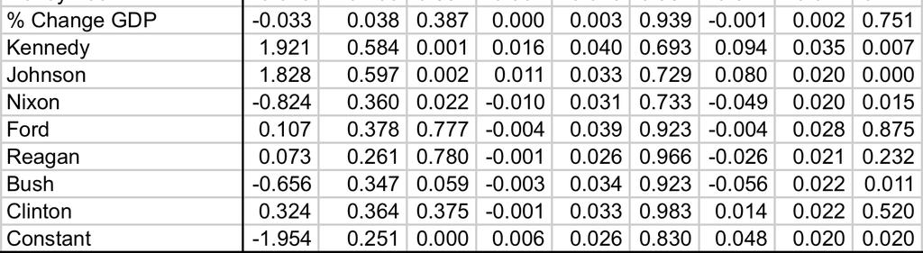
40 Table A1. Endogeneity as a Consequence of Omitted Variable Bias Outcome OLS W Omitted Outcome Outcome Heckman 2-Stage Treatment Selection (Probit) Outcome OLS W Included Outcome Outcome Heckman 2-Stage D (.095) (.217) (.219) (.077) (.128) (.130) Treatment Selection (Probit) X (.047) (.064) (.065) (.054) (.035) (.040) (.041) (.079) W (.035) (.040) (.041) (.077) Z (.055) (.082) Lambda (.139) (.055) (.092) (.082) Constant (.063) (.116) (.117) (.046) (.049) (.069) (.070) (.056) 39

41 Table A2. Complete Model Estimates for Going Public (Canes-Wrone 2001) 40

42 Table A2 (Continued). Complete Model Estimates for Going Public (Canes-Wrone 2001) 41