The following command was executed on their calculator: mean(randnorm(m,20,16))

Transcription

1 8.1- Confidence Intervals: The Basics Introduction How long does a new model of laptop battery last? What proportion of college undergraduates have engaged in binge drinking? How much does the weight of a quarter-pound hamburger at a fast-food restaurant vary after cooking? These are the types of questions we would like to be able to answer. It wouldn t be practical to determine the lifetime of every laptop battery, to ask all college undergraduates about their drinking habits, or to weigh every burger after cooking. Instead, we choose a sample of individuals (batteries, college students, burgers) to represent the population and collect data from those individuals. Our goal in each case is to use a sample statistic to estimate an unknown population parameter. From what we learned in Ch. 4, if we randomly select the sample, we should be able to generalize our results to the population of interest. We cannot be certain that our conclusions are correct a different sample would probably yield a different estimate. Statistical inference uses the language of probability to express the strength of our conclusions. Probability allows us to take chance variation due to random selection or random assignment into account. The following Activity gives you an idea of what lies ahead. Activity: The Mystery Mean Suppose your teacher has selected a Mystery Mean value µ and stored it as M in their calculator. Your task is to work together in pairs to estimate this value. The following command was executed on their calculator: mean(randnorm(m,20,16)) The result was This tells us the calculator chose an SRS of 16 observations from a Normal population with mean M and standard deviation 20. The resulting sample mean of those 16 values was Your group must determine an interval of reasonable values for the population mean µ. Use the result above and what you learned about sampling distributions in the previous chapter. Share your pair s results with the class. Confidence Intervals: The Basics If you had to give one number to estimate an unknown population parameter, what would it be? If you were estimating a population mean μ, you would probably use x. If you were estimating a population proportion p, you might use p. In both cases, you would be providing a point estimate of the parameter of interest. A point estimator is a statistic that provides an estimate of a population parameter. The value of that statistic from a sample is called a point estimate. We learned in Ch. 7 that an ideal point estimator will have no bias and low variability. Since variability is almost always present when calculating statistics from different samples, we must extend our thinking about estimating parameters to include an acknowledgement that repeated sampling could yield different results.

2 Ex: In each of the following settings, determine the point estimator you would use and calculate the value of the point estimate. a. Quality control inspectors want to estimate the mean lifetime μ of the AA batteries produced in an hour at a factory. They select a random sample of 12 batteries during each hour of production and then drain them under conditions that mimic normal use. Here are the lifetimes (in hours) of the batteries from one such sample: b. What proportion p of U.S. high school students smoke? The 2011 Youth Risk Behavioral Survey questioned a random sample of 15,425 students in grades 9 to 12. Of these, 2792 said they had smoked cigarettes at least one day in the past month. The Idea of a Confidence Interval Recall the Mystery Mean Activity. Is the value of the population mean µ exactly ? Probably not. However, since the sample mean is , we could guess that µ is somewhere around How close to is µ likely to be? To answer this question, we must ask another: How would the sample mean x vary if we took many SRSs of size 16 from the population?

3 To estimate the Mystery Mean μ, we can use x = as a point estimate. We don t expect μ to be exactly equal to x so we need to say how accurate we think our estimate is. In repeated samples, the values of x follow a Normal distribution with mean and standard deviation 5. The Rule tells us that in 95% of all samples of size 16, x will be within 10 (two standard deviations) of μ. If x is within 10 points of μ, then μ is within 10 points of x. Therefore, the interval from x 10 to x + 10 will capture μ in about 95% of all samples of size 16. If we estimate that µ lies somewhere in the interval to , we d be calculating an interval using a method that captures the true µ in about 95% of all possible samples of this size. The big idea: The sampling distribution of x tells us how close to μ the sample mean x is likely to be. All confidence intervals we construct will have a form similar to this: Estimate ± Margin of Error Caution: Plausible does not mean the same thing as possible. You could argue that just about any value of a parameter is possible. A plausible value of a parameter is a reasonable or believable value based on the data.

4 There is a trade-off between the confidence level and the amount of information provided by a confidence interval, as the cartoon illustrates. We usually choose a confidence level of 90% or higher because we want to be quite sure of our conclusions. The most common confidence level is 95%. Ex: Two weeks before a presidential election, a polling organization asked a random sample of registered voters the following question: If the presidential election were held today, would you vote for candidate A or candidate B? Based on this poll, the 95% confidence interval for the population proportion who favor candidate A is (0.48, 0.54). PROBLEM: a. Interpret the confidence interval. b. What is the point estimate that was used to create the interval? What is the margin of error? c. Based on this poll, a political reporter claims that the majority of registered voters favor candidate A. Use the confidence interval to evaluate this claim.

5 Activity: The Confidence Intervals Applet 1. Use the default settings: confidence level 95% and sample size n = Click Sample to choose an SRS and display the resulting confidence interval. Did the interval capture the population mean μ (what the applet calls a hit )? Do this a total of 10 times. How many of the intervals captured the population mean μ? Note: So far, you have used the applet to take 10 SRSs, each of size n = 20. Be sure you understand the difference between sample size and the number of samples taken. 3. Reset the applet. Click Sample 25 twice to choose 50 SRSs and display the confidence intervals based on those samples. How many captured the parameter μ? Keep clicking Sample 25 and observe the value of Percent hit. What do you notice? 4. Repeat Step 3 using a 90% confidence level. 5. Repeat Step 3 using an 80% confidence level. 6. Summarize what you have learned about the relationship between confidence level and Percent hit after taking many samples. Interpreting Confidence Levels and Intervals The confidence level is the overall capture rate if the method is used many times. The sample mean will vary from sample to sample, but when we use the method estimate ± margin of error to get an interval based on each sample, C% of these intervals capture the unknown population mean µ.

6 Here s what you should notice: The center x of each interval is marked by a dot. The distance from the dot to either endpoint of the interval is the margin of error. 24 of these 25 intervals (that s 96%) contain the true value of μ. If we took many samples, about 95% of the resulting confidence intervals would capture μ. The confidence level tells us how likely it is that the method we are using will produce an interval that captures the population parameter if we use it many times. The confidence level tells us how likely it is that the method we are using will produce an interval that captures the population parameter if we use it many times. Instead, the confidence interval gives us a set of plausible values for the parameter. We interpret confidence levels and confidence intervals in much the same way whether we are estimating a population mean, proportion, or some other parameter. Ex: The confidence level in the mystery mean example roughly 95% tells us that if we take many SRSs of size 16 from Ms. Mosier s mystery population, the interval x ± 10 will capture the population mean μ for about 95% of those samples. Be sure you understand the basis for our confidence. There are only two possibilities: 1. The interval from to contains the population mean μ. 2. The interval from to does not contain the population mean μ. Our SRS was one of the few samples for which x is not within 10 points of the true μ. Only about 5% of all samples result in a confidence interval that fails to capture μ. Note: We cannot know whether our sample is one of the 95% for which the interval x ± 10 catches μ or whether it is one of the unlucky 5%. The statement that we are 95% confident that the unknown μ lies between and is shorthand for saying, We got these numbers by a method that gives correct results 95% of the time.

7 Ex: The Pew Internet and American Life Project asked a random sample of 2253 U.S. adults, Do you ever use Twitter or another service to share updates about yourself or to see updates about others? Of the sample, 19% said Yes. According to Pew, the resulting 95% confidence interval is (0.167, 0.213). PROBLEM: Interpret the confidence interval and the confidence level. Caution: Confidence intervals are statements about parameters. In the previous example, it would be wrong to say, We are 95% confident that the interval from to contains the sample proportion of U.S. adults who use Twitter. Why? Because we know that the sample proportion, p = 0.19, is in the interval. Likewise, in the mystery mean example, it would be wrong to say that 95% of the values are between and , whether we are referring to the sample or the population. All we can say is, Based on Ms. Mosier s sample, we believe that the population mean is somewhere between and When interpreting a confidence interval, make it clear that you are describing a parameter and not a statistic. And be sure to include context.

8 On Your Own: How much does the fat content of Brand X hot dogs vary? To find out, researchers measured the fat content (in grams) of a random sample of 10 Brand X hot dogs. A 95% confidence interval for the population standard deviation σ is 2.84 to Interpret the confidence interval. 2. Interpret the confidence level. 3. True or false: The interval from 2.84 to 7.55 has a 95% chance of containing the actual population standard deviation σ. Justify your answer.

9 Activity: The Confidence Intervals Applet Why settle for 95% confidence when estimating an unknown parameter? Do larger random samples yield better intervals? 1. Use the default settings: confidence level 95% and sample size n = 20. Click Sample Change the confidence level to 99%. What happens to the length of the confidence intervals? 3. Now change the confidence level to 90%. What happens to the length of the confidence intervals? 4. Finally, change the confidence level to 80%. What happens to the length of the confidence intervals? 5. Summarize what you learned about the relationship between the confidence level and the length of the confidence intervals for a fixed sample size. 6. Reset the applet and change the confidence level to 95%. What happens to the length of the confidence intervals as you increase the sample size? 7. Does increasing the sample size increase the capture rate (percent hit)? Use the applet to investigate.

10 What We ve Seen As the Activity illustrates, the price we pay for greater confidence is a wider interval. If we re satisfied with 80% confidence, then our interval of plausible values for the parameter will be much narrower than if we insist on 90%, 95%, or 99% confidence. But we ll also be much less confident in our estimate. Taking the idea of confidence to an extreme, what if we want to estimate with 100% confidence the proportion p of all U.S. adults who use Twitter? That s easy: we re 100% confident that the interval from 0 to 1 captures the true population proportion! The activity also shows that we can get a more precise estimate of a parameter by increasing the sample size. Larger samples yield narrower confidence intervals. This result holds for any confidence level. Constructing Confidence Intervals Why settle for 95% confidence when estimating a parameter? The price we pay for greater confidence is a wider interval. When we calculated a 95% confidence interval for the mystery mean µ, we started with estimate ± margin of error Our estimate came from the sample statistic x. Since the sampling distribution of x is Normal, about 95% of the values of x will lie within 2 standard deviations (2σ x ) of the mystery mean μ. That is, our interval could be written as: ± 2 5 = x ± 2σ x Properties of Confidence Intervals: The margin of error is the (critical value) (standard deviation of statistic) The user chooses the confidence level, and the margin of error follows from this choice. The critical value depends on the confidence level and the sampling distribution of the statistic. Greater confidence requires a larger critical value The standard deviation of the statistic depends on the sample size n

11 Margin of Error So the margin of error gets smaller when: The confidence level decreases. There is a trade-off between the confidence level and the margin of error. To obtain a smaller margin of error from the same data, you must be willing to accept lower confidence. The sample size n increases. Increasing the sample size n reduces the margin of error for any fixed confidence level. Using Confidence Intervals Wisely Here are two important cautions to keep in mind when constructing and interpreting confidence intervals. 8.2: Estimating a Population Proportion Activity: The Beads Your teacher has a container full of different colored beads. There are 500 beads in total. Your goal is to estimate the actual proportion of red beads in the container. Determine how to use a cup to get a simple random sample of beads from the container. Think this through carefully, because you will get to take only one sample. Form teams of 3 or 4 students. Have one student take an SRS of beads. Separate the beads into two groups: those that are red and those that aren t. Count the number of beads in each group. Determine a point estimate for the unknown population proportion. Find a 95% confidence interval for the parameter p. Consider any conditions that are required for the methods you use.

12 Conditions for Estimating p Before constructing a confidence interval for p, you should check some important conditions: 1. Random: The data should come from a well-designed random sample or randomized experiment. Otherwise, there s no scope for inference to a population (sampling) or inference about cause and effect (experiment). If we can t draw conclusions beyond the data at hand, there s not much point in constructing a confidence interval! Another important reason for random selection or random assignment is to introduce chance into the data-production process. We can model chance behavior with a probability distribution, like the sampling distributions of Ch. 7. The probability distribution helps us calculate a confidence interval %: The procedure for calculating confidence intervals assumes that individual observations are independent. Well-conducted studies that use random sampling or random assignment can help ensure independent observations. However, our formula for the standard deviation of the sampling distribution of p, σ p = p(1 p), acts as if we are sampling with replacement from a n population. That s rarely the case. When sampling without replacement from a finite population, be sure to check that n 1 N. 10 Sampling more than 10% of the population would give a more precise estimate of the parameter p but would require us to use a different formula to calculate the standard deviation of the sampling distribution. 3. Large Counts: The method that we use to construct a confidence interval for p depends on the fact that the sampling distribution of p is approximately Normal. From what we learned in Ch. 7, we can use the Normal approximation to the sampling distribution of p as long as np 10 and n(1 p) 10 In practice, of course, we don t know the value of p. o If we did, we wouldn t need to construct a confidence interval for it! So we cannot check if np and n(1 p) are at least 10. In large random samples, p will tend to be close to p. So we replace p by p in checking the Large Counts condition: o np 10 o n(1 p ) 10

13 Ex: Mr. Vignolini s class wants to construct a confidence interval for the true proportion p of red beads in the container. The class s sample had 107 red beads and 144 white beads. There were 3000 beads in the container. PROBLEM: Check that the conditions for constructing a confidence interval for p are met. Note: What happens if one of the conditions is violated? If the data come from a convenience sample or a poorly designed experiment, there s no point constructing a confidence interval for p. Violation of the Random condition severely limits our ability to make any inference beyond the data at hand. The figure below shows a screen shot from the Confidence Intervals for Proportions applet. We set n = 20 and p = The Large Counts condition is not met because np = 20(0.25) = 5. We used the applet to generate % confidence intervals for p. Only 902 of those 1000 intervals contained p = 0.25, a capture rate of 90.2%. When the Large Counts condition is violated, the capture rate will be lower than the one advertised by the confidence level if the method is used many times. That leaves just the 10% condition when sampling without replacement from a finite population. Large random samples give more precise estimates than small random samples. So randomly selecting more than 10% of a population should be a good thing! Unfortunately, the formula for the standard deviation of p that we developed in Ch. 7, σ p = p(1 p), is not correct when the 10% condition is violated. The formula gives a value that is too large. Confidence intervals based on this formula are longer than they need to be. If many 95% confidence intervals for a population proportion are constructed in this way, more than 95% of them will capture p. The actual capture rate is greater than the reported confidence level when the 10% condition is violated. n

14 On Your Own: In each of the following settings, check whether the conditions for calculating a confidence interval for the population proportion p are met. 1. An AP Statistics class at a large high school conducts a survey. They ask the first 100 students to arrive at school one morning whether or not they slept at least 8 hours the night before. Only 17 students say Yes. 2. A quality control inspector takes a random sample of 25 bags of potato chips from the thousands of bags filled in an hour. Of the bags selected, 3 had too much salt. Constructing a Confidence Interval for p We can use the general formula from Section 8.1 to construct a confidence interval for an unknown population proportion p: statistic (critical value) (standard deviation of statistic) The sample proportion p is the statistics we use to estimate p. When the Independent condition is met, the standard deviation of the sampling distribution of p is σ p = p(1 p) n Since we don t know p, we replace it with the sample proportion p. This gives us the standard error (SE) of the sample proportion: p (1 p ) n When the standard deviation of a statistic is estimated from data, the results is called the standard error of the statistic.

15 Finding a Critical Value How do we find the critical value for our confidence interval? statistic (critical value) (standard deviation of statistic) If the Large Counts condition is met, we can use a Normal curve. To find a level C confidence interval, we need to catch the central area C under the standard Normal curve. To find a 95% confidence interval, we use a critical value of 2 based on the rule. Using Table A or a calculator, we can get a more accurate critical value. Note, the critical value z* is actually 1.96 for a 95% confidence level. Ex:

16 One Sample z Interval for a Population Proportion Once we find the critical value z*, our confidence interval for the population proportion p is statistic (critical value) (standard deviation of statistic) pˆ z * pˆ(1 pˆ) n The resulting interval is sometimes called a one-sample z interval for a population proportion.

17 On Your Own: Alcohol abuse has been described by college presidents as the number one problem on campus, and it is an important cause of death in young adults. How common is it? A survey of 10,904 randomly selected U.S. college students collected information on drinking behavior and alcohol-related problems. The researchers defined frequent binge drinking as having five or more drinks in a row three or more times in the past two weeks. According to this definition, 2486 students were classified as frequent binge drinkers. a. Identify the parameter of interest. b. Check conditions for constructing a confidence interval for the parameter. c. Find the critical value for a 99% confidence interval. Show your method. Then calculate the interval. d. Interpret the interval in context.

18 The Four Step Process We can use the familiar four-step process whenever a problem asks us to construct and interpret a confidence interval. Ex: The Gallup Youth Survey asked a random sample of 439 U.S. teens aged 13 to 17 whether they thought young people should wait to have sex until marriage. Of the sample, 246 said Yes. Construct and interpret a 95% confidence interval for the proportion of all teens who would say Yes if asked this question.

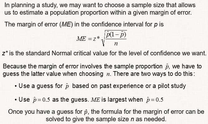
19 Choosing the Sample Size

20 The maximum margin of error would have to be provided if they wanted us to choose a sample size that s appropriate. Ex: A company has received complaints about its customer service. The managers intend to hire a consultant to carry out a survey of customers. Before contacting the consultant, the company president wants some idea of the sample size that she will be required to pay for. One critical question is the degree of satisfaction with the company s customer service, measured on a five-point scale. The president wants to estimate the proportion p of customers who are satisfied (that is, who choose either satisfied or very satisfied, the two highest levels on the five-point scale). She decides that she wants the estimate to be within 3% (0.03) at a 95% confidence level. How large a sample is needed? Problem: Determine the sample size needed to estimate p within 0.03 with 95% confidence. The critical value for 95% confidence is z* = We have no idea about the true proportion p of satisfied customers, so we decide to use p = 0.5 as our guess. Because the company president wants a margin of error of no more than 0.03, we need to solve the equation: margin of error 0.03 Because the company president wants a margin of error of no more than 0.03, we need to solve the equation

21 On Your Own: Refer to the previous example about the company s customer satisfaction survey. a. In the company s prior-year survey, 80% of customers surveyed said they were somewhat satisfied or very satisfied. Using this value as a guess for p, find the sample size needed for a margin of error of 3% at a 95% confidence level. b. What if the company president demands 99% confidence instead? Determine how this would affect your answer to Question Estimating a Population Mean Introduction When we did the Mystery Mean Activity, we got the value of x = from an SRS of size 16. We knew the population distribution was Normal and that its standard deviation was σ = 20. To calculate a 95% confidence interval for μ, we use our familiar formula: statistic ± (critical value) (standard deviation of statistic)

22 The critical value, z* = 1.96, tells us how many standardized units we need to go out to catch the middle 95% of the sampling distribution. Our interval is x ± z σ n = ± = ± 9.8 = (230.99, ) 16 We call such an interval a one-sample z interval for a population mean. This method isn t very useful in practice, however. In most real-world settings, if we don t know the population mean μ, then we don t know the population standard deviation σ either. How do we estimate μ when the population standard deviation σ is unknown? Our best guess for the value of σ is the sample standard deviation sx. Maybe we could use the one-sample z interval for a population mean with sx in place of σ: x ± z s x n When σ is Unknown: The t Distributions When the sampling distribution of x is close to Normal, we can find probabilities involving x by standardizing: x μ z = σ n When we don t know σ, we can estimate it using the sample standard deviation sx. What happens when we standardize? x μ?? = s x n When we standardize based on the sample standard deviation sx, our statistic has a new distribution called a t distribution. It has a different shape than the standard Normal curve: It is symmetric with a single peak at 0, However, it has much more area in the tails.

23 Like any standardized statistic, t tells us how far x is from its mean μ in standard deviation units. There is a different t distribution for each sample size, specified by its degrees of freedom (df). The t Distribution; Degrees of Freedom When we perform inference about a population mean µ using a t-distribution, the appropriate degrees of freedom are found by subtracting 1 from the sample size n, making df = n - 1. We will write the t distribution with n - 1 degrees of freedom as tn-1. When comparing the density curves of the standard Normal distribution and t-distributions, several facts are apparent: The density curves of the t-distributions are similar in shape to the standard Normal curve. The spread of the t-distributions is a bit greater than that of the standard Normal distribution. The t-distributions have more probability in the tails and less in the center than does the standard Normal. As the degrees of freedom increase, the t- density curve approaches the standard Normal curve ever more closely. How to Find the Critical Values of t Table B gives critical values t* for the t-distributions. Each row in the table contains critical values for the t-distribution whose degrees of freedom appear at the left of the row. For convenience, several of the more common confidence levels C are given at the bottom of the table. By looking down any column, you can check that the t-critical values approach the Normal critical values z* as the degrees of freedom increase. When you use Table B to determine the correct value of t* for a given confidence interval, all you need to know are the confidence level C and the degrees of freedom (df). Unfortunately, Table B does not include every possible sample size. When the actual df does not appear in the table, use the greatest df available that is less than your desired df. This guarantees a wider confidence interval than you need to justify a given confidence level. Better yet, use technology to find an accurate value of t* for any df.

24 Ex: Problem: What critical value t* from Table B should be used in constructing a confidence interval for the population mean in each of the following settings? a. A 95% confidence interval based on an SRS of size n = 12. Solution: In Table B, we consult the row corresponding to df = 12-1 = 11. We move across that row to the entry that is directly above 95% confidence level on the bottom of the chart. The desired critical value is t* = b. A 90% confidence interval from a random sample of 48 observations. Solution: With 48 observations, we want to find the t* critical value for df = 48-1 = 47 and 90% confidence. There is no df = 47 row in Table B, so we use the more conservative df = 40. The corresponding critical value is t* = On Your Own: Use Table B to find the critical value t* that you would use for a confidence interval for a population mean μ in each of the following settings. If possible, check your answer with technology. a. A 96% confidence interval based on a random sample of 22 observations. b. A 99% confidence interval from an SRS of 71 observations. Conditions for Estimating μ As with proportions, you should check some important conditions before constructing a confidence interval for a population mean.

25 What about Small Samples? Larger samples improve the accuracy of critical values from the t distributions when the population is not Normal. This is true for two reasons: 1. The sampling distribution of x for large sample sizes is close to Normal. 2. As the sample size n grows, the sample standard deviation sx will give a more accurate estimate of σ. This is important because we use s x in place of σ when doing calculations. n n The Normal/Large Sample condition is obviously met if we know that the population distribution is Normal or that the sample size is at least 30. What if we don t know the shape of the population distribution and n < 30? In that case, we have to graph the sample data. Our goal is to answer the question, Is it reasonable to believe that these data came from a Normal population? How should graphs of data from small samples look if the population has a Normal distribution? Let s use the calculator to simulate choosing random samples of size n = 20 from a Normal distribution with μ = 100 and σ = 15 and then to plot the data as a box-and-whisker plot. What do you expect the sample distribution to look like? Did you expect that a random sample from a Normal population would yield a graph that looked Normal? Unfortunately, that s usually not the case. The figure below shows boxplots from three different SRSs of size 20 chosen. The left-hand graph is skewed to the right. The right-hand graph shows three outliers in the sample. Only the middle graph looks symmetric and has no outliers. CAUTION: As the last slide shows, it is very difficult to use a graph of sample data to assess the Normality of a population distribution. If the graph has a skewed shape or if there are outliers present, it could be because the population distribution isn t Normal. Skewness or outliers could also occur naturally in a random sample from a Normal population. To be safe, you should only use a t-distribution for small samples with no outliers or strong skewness.

26 Ex: PROBLEM: Determine if we can safely use a t* critical value to calculate a confidence interval for the population mean in each of the following settings. a. To estimate the average GPA of students at your school, you randomly select 50 students from classes you take. Figure 8.14(a) is a histogram of their GPAs. b. How much force does it take to pull wood apart? Figure 8.14(b) shows a stemplot of the force (in pounds) required to pull apart a random sample of 20 pieces of Douglas fir. c. Suppose you want to estimate the mean SAT Math score at a large high school. Figure 8.14(c) is a boxplot of the SAT Math scores for a random sample of 20 students at the school.

27 Constructing a Confidence Interval for μ When the conditions for inference are satisfied, the sampling distribution for x has roughly a Normal distribution. Because we don t know σ, we estimate it by the sample standard deviation s x. To construct a confidence interval for µ, Replace the standard deviation of x by its standard error in the formula for the one-sample z interval for a population mean. Use critical values from the t-distribution with n - 1 degrees of freedom in place of the z critical values. That is, statistic ± (critical value) (standard deviation of statistic) = x ± t s x n One Sample t Interval for a Population Mean The one-sample t interval for a population mean is similar in both reasoning and computational detail to the one-sample z interval for a population proportion

28 Ex: Environmentalists, government officials, and vehicle manufacturers are all interested in studying the auto exhaust emissions produced by motor vehicles. The major pollutants in auto exhaust from gasoline engines are hydrocarbons, carbon monoxide, and nitrogen oxides (NOX). Researchers collected data on the NOX levels (in grams/mile) for a random sample of 40 light-duty engines of the same type. The mean NOX reading was and the standard deviation was Problem: a. Construct and interpret a 95% confidence interval for the mean amount of NOX emitted by light-duty engines of this type. State: We want to estimate the true mean amount µ of NOX emitted by all light-duty engines of this type at a 95% confidence level. Plan: If the conditions are met, we should use a one-sample t interval to estimate µ. Random: The data come from a random sample of 40 engines from the population of all light-duty engines of this type. 10%?: We are sampling without replacement, so we need to assume that there are at least 10(40) = 400 light-duty engines of this type. Large Sample: We don t know if the population distribution of NOX emissions is Normal. Because the sample size is large, n = 40 > 30, we should be safe using a t distribution. Do: From the information given, x = g/mi and sx = g/mi. To find the critical value t*, we use the t distribution with df = 40-1 = 39. Unfortunately, there is no row corresponding to 39 degrees of freedom in Table B. We can t pretend we have a larger sample size than we actually do, so we use the more conservative df = 30. = (1.1599, ) Conclude: We are 95% confident that the interval from to grams/mile captures the true mean level of nitrogen oxides emitted by this type of light-duty engine. b. The Environmental Protection Agency (EPA) sets a limit of 1.0 gram/mile for average NOX emissions. Are you convinced that this type of engine violates the EPA limit? Use your interval from (a) to support your answer.

29 Note: Now that we ve calculated our first confidence interval for a population mean μ, it s time to make a simple observation: Inference for proportions uses z; inference for means uses t That s one reason why distinguishing categorical from quantitative variables is so important. Here is another example, this time with a smaller sample size. Ex: A manufacturer of high-resolution video terminals must control the tension on the mesh of fine wires that lies behind the surface of the viewing screen. Too much tension will tear the mesh, and too little will allow wrinkles. The tension is measured by an electrical device with output readings in millivolts (mv). Some variation is inherent in the production process. Here are the tension readings from a random sample of 20 screens from a single day s production: Construct and interpret a 90% confidence interval for the mean tension μ of all the screens produced on this day. State: We want to estimate the true mean tension μ of all the video terminals produced this day with 90% confidence. Plan: If the conditions are met, we should use a one-sample t interval to estimate µ. Random: We are told that the data come from a random sample of 20 screens produced that day. 10%?: Because we are sampling without replacement, we must assume that at least 10(20) = 200 video terminals were produced this day. Large Sample: Because the sample size is small (n = 20), we must check whether it s reasonable to believe that the population distribution is Normal. So we examine the sample data. Figure 8.15 shows (a) a dotplot, (b) a boxplot, and (c) a Normal probability plot of the tension readings in the sample. Neither the dotplot nor the boxplot shows strong skewness or any outliers. The Normal probability plot looks roughly linear. These graphs give us no reason to doubt the Normality of the population.

30 Do: We used our calculator to find the mean and standard deviation of the tension readings for the 20 screens in the sample: x = mv and sx = mv. To find the critical value t*, we use the t distribution with df = 20-1 = 19. t = = (292.32, ) Conclude: We are 90% confident that the interval from to mv captures the true mean tension in the entire batch of video terminals produced that day. On Your Own: Biologists studying the healing of skin wounds measured the rate at which new cells closed a cut made in the skin of an anesthetized newt. Here are data from a random sample of 18 newts, measured in micrometers (millionths of a meter) per hour: Calculate and interpret a 95% confidence interval for the mean healing rate μ.

31 Choosing a Sample Size A wise user of statistics never plans data collection without planning the inference at the same time. You can arrange to have both high confidence and a small margin of error by taking enough observations. When the population standard deviation σ is unknown and conditions are met, the C % confidence interval for μ is x ± t s x n where t* is the critical value for confidence level C and degrees of freedom df = n 1. The margin of error (ME) of the confidence interval is ME = t s x n To determine the sample size for a desired margin of error, it makes sense to set the expression for ME less than or equal to the specified value and solve the inequality for n. There are two problems with this approach: 1. We don t know the sample standard deviation sx because we haven t produced the data yet. 2. The critical value t* depends on the sample size n that we choose. The second problem is more serious. To get the correct value of t*, we need to know the sample size. But that s what we re trying to find! There is no easy solution to this problem. One alternative (the one we recommend!) is to come up with a reasonable estimate for the population standard deviation s from a similar study that was done in the past or from a small-scale pilot study. By pretending that s is known, we can use the one-sample z interval for μ: x ± z σ n Using the appropriate standard Normal critical value z* for confidence level C, we can solve for n. Here is a summary of this strategy: z σ n ME

32 We determine a sample size for a desired margin of error when estimating a mean in much the same way we did when estimating a proportion. Ex: Researchers would like to estimate the mean cholesterol level µ of a particular variety of monkey that is often used in laboratory experiments. They would like their estimate to be within 1 milligram per deciliter (mg/dl) of the true value of µ at a 95% confidence level. A previous study involving this variety of monkey suggests that the standard deviation of cholesterol level is about 5 mg/dl. Problem: Obtaining monkeys is time-consuming and expensive, so the researchers want to know the minimum number of monkeys they will need to generate a satisfactory estimate. Solution: For 95% confidence, z* = We will use σ = 5 as our best guess for the standard deviation of the monkeys cholesterol level. Set the expression for the margin of error to be at most 1 and solve for n : Because 96 monkeys would give a slightly larger margin of error than desired, the researchers would need 97 monkeys to estimate the cholesterol levels to their satisfaction. On Your Own: Administrators at your school want to estimate how much time students spend on homework, on average, during a typical week. They want to estimate μ at the 90% confidence level with a margin of error of at most 30 minutes. A pilot study indicated that the standard deviation of time spent on homework per week is about 154 minutes. How many students need to be surveyed to meet the administrators goal? Show your work.

33