POLITECNICO DI MILANO

Transcription

1 POLITECNICO DI MILANO Scuola di Ingegneria Industriale e dell Informazione Tesi di Laurea Magistrale in Ingegneria Biomedica Development of a method for the in vivo assessment of aortic root local mechanical properties Supervisor: Prof. Ing. Emiliano VOTTA Co-supervisors: Prof.Ing. Peter JOHANSEN Ing. Alessandro CAIMI Author: Laura MARELLI Matricola: Anno Accademico 2017/2018

2 Contents Abstract III Sommario XII 1. The aortic root The heart Anatomy and physiology of the heart Anatomy and physiology of the aortic root Aortic valve Aortic wall Aortic root dynamics Pathologies of the aortic root Ascending Thoracic Aortic Aneurysm Biomechanical properties of ATAA Diagnosis State of the art Experimental studies on local aortic root biomechanics In vitro studies In vivo studies In silico studies on aortic tissue biomechanics Stress analysis Strain analysis Aortic root model Objective Materials and methods Acquisition of medical images Reconstruction of the 3D model 45 I

3 3.3. Stress Calculation Computation of strains Mechanical properties estimation Sensitivity analysis Validation Results and discussion Validation Curvatures Stresses Strains Material properties Tracking function Conclusions Application to in vivo data from an animal model D geometry Stresses Strains Aortic root shape changes Material properties Application on a clinical case D geometry Stresses Strains Aortic root shape changes Material properties Conclusions 96 5 Conclusions Limits and Future Developments 98 Bibliography 101 APPENDIX 104 II

4 Abstract Introduction The aortic root is the functional-anatomical unit that connects the left ventricle to the thoracic ascending aorta and that supports the constitutive elements of the aortic valve. Its main components are the aortic annulus, the interleaflet triangles (ILTs), the three sinuses of Valsalva, and the sinotubular junction (Figure A). The aortic annulus represents the inlet from the left ventricular outflow tract into the aortic root, where the local lower points of the valve leaflets are inserted. The interleaflet triangles are a crown-shaped structure delimited proximally by the aorto-ventricular junction and distally by the profile of the leaflet insertion on the aortic wall. The three sinuses of Valsalva are the three lobes of the aortic wall corresponding each one to a valve leaflet and representing the reason for the bulb shape structure of the aortic root. The left sinus, right sinus and non-coronary sinus acquire their names from the arteries originating from them. The sinotubular junction is the connection between the sinuses of Valsalva and the ascending aorta. III

5 Figure A: Aortic root structures: the annulus (in green), the interleaflet triangles (red), the ventriculo-arotic junctions (yellow), the sinotubular junctions (blue)[1] In physiologic conditions, during the cardiac cycle the aortic root substructures deform in different modes in order to maximize ejection, to optimize the trans-valve fluid dynamics and to reduce the stresses on the valve leaflets with an optimal load distribution. The upper portion of the aortic root is subjected to aortic pressure changes. It expands during systole allowing the leaflets to retract and open. The proximal part is exposed to ventricular pressure. It expands as the ventricle fills and it contracts during peak systole, so that the distance the leaflets have to travel to coat decreases. This aortic root action helps in reducing stresses present on valve leaflets.[2] State of the art Understanding aortic root mechanical behaviour is pivotal in clinics. Anomalies in aortic wall mechanical properties, if detected in vivo and non-invasively, could be exploited as a surrogate measure of pathologies affecting the structure of aortic wall tissue. There are studies (e.g., [3] [4]) that investigated the material characteristics and the dimensional changes of the aortic root during the cardiac cycle. Many of these studies investigated in vitro tissue samples. However, once the tissue sample is extracted from the body, due to the presence of a different environment and conditions, its chemical and structural properties could change, affecting the results of an in vitro mechanical characterization. Moreover, methods based on ex vivo inspections cannot be translated to the analysis of tissue IV

6 mechanical properties in humans as a mean to support diagnosis. Motivated by these limitations, other studies investigated aortic root properties in vivo through the insertion of radio-markers. Doubtless, these approaches are invasive and cannot be envisioned as a mean to diagnose anomalies. Therefore, a computational approach through finite element methods, starting from in vivo imaging techniques, could be a significant solution for the non-invasive detection of local material properties of the aortic wall. Studies already adopted computational solutions for the detection of tissue local material properties, through the computation of stresses thanks to the calculation of local curvatures and detection of local displacement using tracking methods [5]. However, no study investigated, through a computational approach, aortic root material properties in vivo. The goal of this work is the detection of local aortic root material properties through a finite element reverse engineering method. Materials and methods The developed method to assess in vivo mechanical properties consists of five steps (Figure B): a) Images acquisition b) 3D aortic root reconstruction based on acquired images c) Detection of local in vivo stresses along the aortic root wall d) Detection of local in vivo strains along the aortic root wall e) Based on the strains-stresses curves, material aortic root properties detection The core of this pipeline consists in steps c) and d), which were implemented based on the assumption that in general the aortic wall can be reconstructed in the form of a triangulated 3D surface. In step c), stresses were calculated based on the thin wall hypothesis, hence through the local application of the Laplace law, where circumferential and axial stresses are proportional to the intraluminal pressure and inversely proportional to the respective local curvatures and thickness. In general, wall thickness cannot be measured reliably from medical images; hence, it was assumed based on the literature. Different thickness values assumed for different aortic root sections. Ventricular and aortic pressure were applied on the aortic root base and on the area starting from Valsalva sinuses to ascending aorta tract, respectively. Pressure data were either experimentally measured or assumed based on the literature. Local curvatures were quantified following [6] briefly, for a given node of interest P in the V

7 triangulated surface a local patch was defined, which encompassed P and any node falling within two edges from P on the grid. The geometry of the local patch was approximated by a quadratic polynomial function, whose curvature tensor could be computed analytically to then project the tensor on any relevant direction, i.e., in our case, the axial and circumferential direction of the aortic wall. Figure B: Schematic representation of the developed algorithm for the study of aortic root mechanical properties In step d), Green-Lagrange strains were computed through the combination of a tracking algorithm and a finite element approach. Briefly, a regular pattern of 9-node quadratic corotational shell elements was defined on the aortic wall at end-diastole, i.e., the time-point of minimal aortic pressure. For each shell element, nodes were chosen among the nodes of the triangulated surface representing the aortic wall. These nodes were tracked frame-byframe on the medical images through a previously developed algorithm [7]: for every point of interest at time t, the algorithm identifies the new position at time t+1 by minimizing a definite positive cost function that is proportional to changes in position and in local curvature from time t to time t+1. The time-dependent displacements of the tracked nodes was interpreted as the set of time-dependent nodal-displacements to be imposed to the 9- VI

8 node co-rotational shell elements. The formulation of the 9-node co-rotational shell elements was borrowed from the Li and colleagues [8], and it was exploited to obtain i) the displacement field within the element Lagrangian shape functions and ii) the deformation field through the partial derivatives of the displacement field. In step e), the strain and stress data computed at the center of each shell element and at different time-points are used as if these were yielded by a biaxial mechanical test. Hence, these are fitted to identify the local value of the constitutive parameters of the May Newman constitutive model, which captures the anisotropic hyperelastic mechanical properties of wall tissue: W = c 0 (e Q 1), with Q = c 1 (I 1 3) 3 + c 2 (α 1) where c 0 is the stiffness parameters with dimensions of Pascal and c 1 and c 2 are no-dimensional parameters. The algorithm was first validated vs. a finite element phantom [9]: previously performed finite element simulations of aortic root structural mechanics were exploited to extract the loaded configuration of the wall at different time-points throughout the cardiac cycle. Circumferential and axial strains and stresses computed at 36 different positions over the wall by the approach herein developed were compared vs. the strains and the stresses computed directly by the finite element simulation at the same spots. Second, the algorithm was applied to real computed tomography (CT) and pressure data acquired on a healthy pig. CT scans were obtained at the Department of Cardiothoracic & Vascular Surgery, Aarhus University Hospital, Aarhus, Denmark. The acquisition of the images was monitored step by step, preparation of the pig included. Two series of CT scans were acquired through a SIEMENS machine. The series of data collected covered the all cardiac cycle, with an acquisition time resolution of corresponding to 20 time points. 40 transverse image-planes were acquired along the all aortic root length. Aortic and ventricular pressures were measured through catheters. Third, the algorithm was applied to CT scans of a human patient affected by aortic valve stenosis. Regarding the clinical case, 202 images were obtained for 20 time points along the cardiac cycle. For obvious reasons, pressure direct measurements were not available. Hence, pressure data from the literature were used, which were characterized by a peak aortic pressure of 120 mmhg. In order to cope with the uncertainty regarding this assumption, analyses were carried out also by increasing and decreasing pressure values by 10%, thus obtaining aortic pressure waves with peak values of 132 and 108 mmhg, respectively. VII

9 When dealing with real CT scans, images were processed by the following pipeline: image contrast was increased, the 3D geometry was reconstructed through a marching cube algorithm implemented in Python (Python Software Foundation. Python Language Reference, version 2.7), setting a value of 130 for the isovalue that corresponded to aortic wall tissue. The corresponding isosurfaces were exported as.stl files containing the 3D triangulated surface of the whole pig chest:.stl files were imported in Meshmixer (Autodesk, Inc) to regularize the triangulated surfaces and to remove the anatomical structures surrounding the root. Results and discussion Using the phantom model, each algorithm section was validated. The validity of the tracking function in the detection of the correct nodes position was tested knowing the node-to-node correspondence for each frame of the phantom model. An error of 13 % was give. However, missed nodes belonged to the same triangular mesh element. Stresses and strains obtained as algorithm output were compared with the ones of the original simulations. For the majority of the shells, a same pattern was identified within the two waves during the cardiac cycle (30 over 36 for circumferential stresses; 19 over 36 for axial stresses; 23 over 36 for circumferential strain; 26 over 36 for axial strains). In these cases, correspondent systolic and diastolic phases and maximum and minimum peaks were detected. As final proof of the algorithm validity, the average of the Young s moduli for each shell was calculated and compared with the original one. A maximum error of 3 % was obtained. Algorithm application on the animal model permitted to characterize every aortic root section behaviour during the cardiac cycle and the definition of local material properties. At peak systolic phase, stresses were found higher at the base (with the first May Newman model c Kpa) and at the sinobular junction (17.96 Kpa). Within the sinuses the highest stress value was reached by the right sinus (16.94 Kpa) and the lowest one by the left sinus (12.79 Kpa). From strains detection during the cardiac cycle it was possible to define the different expansion and contraction modes. Maximum expansion raised at one third of ejection and in particular it was reached by the ascending aorta (21.21 %). The base started its expansion before the other structures. The left and right sinuses underwent higher expansion (21.59 % and % respectively) with respect to the non-coronary one (5.79 %). Considering axial strains as elongation, if positive, and shortening, if negative, all VIII

10 Base - stj difference structures presented elongation during the systolic phase with the exception of the base. This opposite action of the base could be caused by left ventricle influence reducing its volume during ejection. Within longitudinal levels, highest axial strain (18.51 %) was present for the base rather than the other structure. This could be a consequence of the base attachment to the left ventricle and to an anchored position of the other structures. Aortic root shape changes from a cone-shape structure to a more cylindrical one, during the cardiac cycle, as described in Lansac s et al. [3] study were confirmed (Figure C). Moreover, asymmetry in material properties within the different structures was obtained, i.e. the right and noncoronary sinus showing similar stiffness ( Kpa and Kpa) and the left one being more compliant ( Kpa) [10]. Difference within base and sinotubular junction level 30% 25% 20% 15% 10% 5% 0% 0,1 0,5 0,8 1,2 1,6 2,0 2,4 2,8 3,2 3,6 4,0 Time [s] Figure C: relative change in the difference between sinotubular junction and aortic root base indicating aortic root shape changes in the animal model. Considering the clinical case, due to the presence of more noise and to uncertainties regarding patient parameters at acquisition time, detection of modes of deformation during the cardiac cycle was more difficult. Similarities and differences within the animal model were encountered. Also in this case maximum stress was reached by the base (52.90 Kpa for a peak pressure of 120 mmhg). However, the sinotubular junction presented the lower value of stress (8.39 Kpa for a peak pressure of 120 mmhg). Equally to the animal mode, the right and left sinus presented similar circumferential strain values (3.74 % and 4.89 % at peak systolic frame respectively); while the non-coronary sinus presented slightly lower values (1.77 %). However, right and left sinuses underwent expansion during systolic phase as in the animal model case. At the contrary, non-coronary sinus underwent contraction during IX

11 Base -stj difference the same phase. The base also presented highest strain values in axial direction (peak strain at %). However, in this case, it presented highest strain values also in the circumferential one (peak strain at %), contrary to the animal case. An aortic root shape change during the cardiac cycle was notices also in this case. Nonetheless, in this case the initial cone-shape resulted reversed with the sinotubular junction circumference larger than the base one (Figure D). Similarly to the animal model, asymmetry within mechanical properties was detected. Although the base resulted the stiffest structure (with the first May Newman coefficient c0 of Kpa for a peak pressure value of 120 mmhg), sinuses presented different order of stiffness within each other. The left sinus was the stiffest one ( Kpa for a peak pressure value of 120 mmhg) and the right sinus the most compliant (417.3 Kpa for a peak pressure value of 120 mmhg). All structures, with the exception of the right sinus, were found stiffer than the ones in the animal case. Moreover, they resulted also more anisotropic. Differences within base and sinotubular junction 0% -5% -10% -15% -20% 0,1 0,5 0,8 1,2 1,6 2,0 2,4 2,8 3,2 3,6 4,0 Time [s] Figure D: relative change in the difference between sinotubular junction and aortic root base indicating aortic root shape changes in the clinical case. Conclusions An algorithm for detection of local material properties was developed. In literature, anybody provided an identification of in vivo local aortic root material properties. After a first validation phase, the algorithm was applied on an animal model, with controlled parameters during images acquisition, and on a clinical case, with many uncertainties regarding patient clinical state and parameters. Through the animal model, local mechanical behaviour of the aortic root could be defined. The different aortic root modes during the cardiac cycle and the X

12 asymmetry within material properties of the different structures were almost equivalent to data found in literature. Regarding the clinical case, different properties were obtained. This could be due to the pathology affecting the patient or to artefacts during images acquisition and the lack of proper patient-specific information. This method provides an estimation of local material properties that can be used in order to better define surgical techniques simulations. An interesting development of this algorithm could be its use as a tool for diagnosis detection or patient-specific prosthesis design. However, much more effort should be implemented in order to provide defined local material properties estimation in a clinical prospective. Non-invasive methods for intraluminal pressure measurements and a reduction of noise due to patient movement should be taken into consideration. Moreover, a wider set of data should be considered to provide higher robustness to the work. XI

13 Sommario Introduzione La radice aortica è l'unità funzionale-anatomica che collega il ventricolo sinistro all'aorta ascendente toracica e che supporta gli elementi costitutivi della valvola aortica. I suoi componenti principali sono l'anulus aortico, i triangoli interleaflet (ILT), i tre seni di Valsalva e la giunzione sinotubulare (Figura A). L'anulus aortico rappresenta l'ingresso dal tratto di efflusso ventricolare sinistro nella radice aortica, dove sono inseriti i punti inferiori locali dei foglietti valvolari. I triangoli interleaflet sono una struttura a forma di corona delimitata prossimalmente dalla giunzione aorto-ventricolare e distalmente dal profilo dell'inserzione dei foglietti valvolari sulla parete aortica. I tre seni di Valsalva sono i tre lobi della parete aortica corrispondenti ciascuno a un volantino valvolare e rappresentano la ragione della struttura a forma di bulbo della radice aortica. Il seno sinistro, il seno destro e il seno non coronarico acquisiscono i loro nomi dalle arterie che originano da essi. La giunzione sinotubulare è la connessione tra i seni di Valsalva e l'aorta ascendente. XII

14 Figura A: strutture della radici aortiche: l'anulus (in verde), i triangoli interleaflet (rosso), le giunzioni aorto-ventricolari (giallo), le giunzioni sinotubulari (blu) [1] In condizioni fisiologiche, durante il ciclo cardiaco le sottostrutture della radice aortica si deformano in modi diversi al fine di massimizzare l'eiezione, per ottimizzare la fluidodinamica trans-valvolare e per ridurre gli stress sui foglietti della valvola attraverso una distribuzione ottimale del carico. La porzione superiore della radice è soggetta a cambiamenti di pressione aortica. Si espande durante la sistole permettendo ai volantini di ritrarsi e aprirsi. La parte prossimale è esposta alla pressione ventricolare. Si espande quando il ventricolo si riempie e si contrae durante il picco sistolico, in modo che la distanza che i foglietti devono percorrere per ridurre il rivestimento. Questa azione della radice aortica aiuta a ridurre gli stress presenti sui volantini delle valvole. [2] Stato dell arte Capire il comportamento meccanico della radice aortica è cruciale dal punto di vista clinico. Anomalie nelle proprietà meccaniche della parete aortica, se rilevate in vivo e non in modo invasivo, potrebbero essere sfruttate come misure di supporto per la diagnosi di patologie che influenzano la struttura del tessuto della parete aortica. Ci sono studi (ad es. [3] [4]) che hanno studiato le caratteristiche del materiale e le variazioni dimensionali della radice aortica durante il ciclo cardiaco. Molti di questi studi hanno analizzato campioni di tessuto in vitro. Tuttavia, una volta che il campione di tessuto viene estratto dal corpo, a causa della presenza di un ambiente e di condizioni differenti, le sue proprietà chimiche e strutturali potrebbero cambiare, influenzando i risultati di una caratterizzazione meccanica in vitro. Inoltre, i XIII

15 metodi basati su ispezioni ex vivo non possono essere utilizzati per l analisi delle proprietà meccaniche dei tessuti nell'uomo come mezzo per supportare la diagnosi. Motivati da questi limiti, altri studi hanno valutato le proprietà delle radici aortiche in vivo attraverso l'inserimento di radiomarkers. Indubbiamente, questi approcci sono invasivi e non possono essere immaginati come un mezzo per diagnosticare anomalie. Pertanto, un approccio computazionale attraverso i metodi agli elementi finiti, partendo da tecniche di imaging in vivo, potrebbe essere una soluzione significativa per il rilevamento non invasivo delle proprietà locali del materiale della parete aortica. Gli studi hanno già adottato soluzioni computazionali per il rilevamento delle proprietà locali dei tessuti, grazie al calcolo degli sforzi misurati attraverso la rilevazione delle curvature locali e al rilevamento degli spostamenti locali utilizzando metodi di localizzazione [5]. Tuttavia, nessuno studio ha valutato, attraverso un approccio computazionale, le proprietà del materiale della radice aortica in vivo. L'obiettivo di questo lavoro è il rilevamento delle proprietà locali del materiale della radice aortica attraverso un metodo di reverse engineering agli elementi finiti. Materiali e metodi Il metodo sviluppato per valutare le proprietà meccaniche in vivo è caratterizzato da cinque fasi (Figura B): a) Acquisizione di immagini b) Ricostruzione 3D della radice aortica basata su immagini acquisite c) Rilevazione di sforzi locali in vivo lungo la parete della radice aortica d) Rilevazione di deformazioni locali in vivo lungo la parete della radice aortica e) Rilevamento delle proprietà della radice aortica del materiale, In base alle curve deformazioni-sforzo Il nucleo di questa sequenza di fasi consiste nei passaggi c) e d), che sono stati implementati sulla base dell'assunzione che in generale la parete aortica può essere ricostruita sotto forma di una superficie 3D triangolata. Nella fase c), le sollecitazioni sono state calcolate in base all'ipotesi della parete sottile, quindi attraverso l'applicazione locale della legge di Laplace, dove le tensioni circonferenziali e assiali sono proporzionali alla pressione intraluminale e inversamente proporzionali alle rispettive curvature e spessori locali. In generale, lo spessore delle pareti non può essere misurato in modo affidabile dalle immagini mediche; quindi, è stato assunto in base alla letteratura. Diversi valori di spessore sono stati assunti per diverse sezioni di XIV

16 radice aortica. Pressione ventricolare e aortica sono state applicate alla base della radice aortica e all area che inizia dai seni di Valsalva e finisce al tratto ascendente dell'aorta, rispettivamente. I dati sulla pressione sono stati misurati sperimentalmente o ipotizzati in base alla letteratura. Le curvature locali sono state quantificate seguendo [6]: in breve, per un dato nodo di interesse P nella superficie triangolare è stato definita una patch locale, che comprendeva P e qualsiasi nodo che si trovava entro due bordi da P sulla griglia. La geometria della patch locale è stata approssimata da una funzione polinomiale quadratica, il cui tensore di curvatura potrebbe essere calcolato analiticamente per poi proiettare il tensore su qualsiasi direzione pertinente, vale a dire, nel nostro caso, la direzione assiale e circonferenziale della parete aortica. Figura B: Rappresentazione schematica dell'algoritmo sviluppato per lo studio delle proprietà meccaniche della radice aortica Nella fase d), le deformazioni di Green-Lagrange sono state calcolate attraverso la combinazione di un algoritmo di tracciamento e un approccio ad elementi finiti. In breve, un modello regolare di elementi shell co-rotazionale quadratico a 9 nodi è stato definito sulla parete aortica a fine diastole, ovvero l istante temporale in cui la pressione aortica è minima. Per ciascun elemento della shell, i nodi sono stati selezionati tra i nodi della superficie triangolare che rappresenta la parete aortica. Questi nodi sono stati tracciati fotogramma per fotogramma sulle immagini mediche attraverso un algoritmo precedentemente sviluppato XV

17 [7]: per ogni punto di interesse al tempo t, l'algoritmo identifica la nuova posizione al tempo t + 1 minimizzando una funzione di errore definita positivamente, proporzionale alle variazioni di posizione e alla curvatura locale dal tempo t al tempo t + 1. Gli spostamenti dipendenti dal tempo dei nodi tracciati sono stati interpretati come l'insieme di spostamenti nodali dipendenti dal tempo da imporre agli elementi shell co-rotativi a 9 nodi. La formulazione degli elementi shell co-rotazionali a 9 nodi è stata presa in prestito da Li e colleghi [8], ed è stata sfruttata per ottenere i) il campo di spostamento all'interno delle funzioni di forma di Lagrange e ii) il campo di deformazione attraverso le derivate parziali del campo di spostamento. Nella fase e), i dati di sforzo e deformazione calcolati al centro di ciascun elemento shell e in diversi istanti temporali vengono utilizzati come se fossero stati ottenuti da un test meccanico biassiale. Quindi, una stima delle proprietà meccaniche locali è stata possibile mediante il modello costitutivo di May Newman [11], che cattura le proprietà meccaniche iperelastiche anisotropiche del tessuto: W = c 0 (e Q 1), dove Q = c 1 (I 1 3) 3 + c 2 (α 1). c 0 è il parametro indicante la rigidità con dimensioni in Pascal e c 1 and c 2 sono parametri non dimensionali. L'algoritmo è stato prima validato mediante un fantoccio a elementi finiti [9]: le simulazioni a elementi finiti della meccanica strutturale della radice aortica eseguite in precedenza sono state sfruttate per estrarre la configurazione carica della parete in diversi istanti temporali durante il ciclo cardiaco. Le deformazioni e gli sforzi circonferenziali e assiali calcolati in 36 diverse posizioni sulla parete mediante l'approccio qui sviluppato sono stati confrontati con le deformazioni e gli sforzi calcolati direttamente dalla simulazione degli elementi finiti negli stessi punti. In secondo luogo, l'algoritmo è stato applicato a immagini in vivo di tomografia computerizzata (CT) e ai dati di pressione acquisiti su un maiale sano. Le scansioni CT sono state ottenute presso il Dipartimento di Chirurgia Cardiotoracica e Vascolare, Aarhus University Hospital, Aarhus, Danimarca. L'acquisizione delle immagini è stata monitorata passo dopo passo, preparazione del maiale incluso. Due serie di scansioni CT sono state acquisite tramite una macchina SIEMENS. La serie di dati raccolti copriva tutto il ciclo cardiaco, con una risoluzione temporale di acquisizione di 0,065 corrispondente a 20 punti temporali. 40 piani di immagine trasversali sono stati acquisiti lungo tutta la lunghezza della radice aortica. Le pressioni aortiche e ventricolari sono state misurate tramite cateteri. XVI

18 In terzo luogo, l'algoritmo è stato applicato alle scansioni TC di un paziente umano affetto da stenosi valvolare aortica. Per quanto riguarda il caso clinico, sono state ottenute 202 immagini per 20 punti temporali lungo il ciclo cardiaco. Per ovvi motivi, le misurazioni dirette della pressione non erano disponibili. Quindi, sono stati utilizzati i dati di pressione dalla letteratura, che erano caratterizzati da una pressione aortica di picco di 120 mmhg. Per far fronte all'incertezza su questa ipotesi, le analisi sono state effettuate anche aumentando e diminuendo i valori di pressione del 10%, ottenendo così le onde di pressione aortica con valori di picco rispettivamente di 132 e 108 mm Hg. Per quanto riguarda scansioni CT in vivo, le immagini sono state elaborate con la seguente sequenza: il contrasto dell'immagine è stato aumentato, la geometria 3D è stata ricostruita attraverso un algoritmo di marching cube implementato in Python (Python Software Foundation, Python Language Reference, versione 2.7), impostando un valore di 130 per l'isovalue che corrispondeva al tessuto della parete aortica. Le corrispondenti isosuperfici sono state esportate come file.stl contenenti la superficie triangolare 3D del petto di maiale intero: i file.stl sono stati importati in Meshmixer (Autodesk, Inc) per regolarizzare le superfici triangolate e rimuovere le strutture anatomiche che circondano la radice. Risultati e discussione Usando il fantoccio, ogni sezione dell'algoritmo è stata validata. La validità della funzione di tracciamento nel rilevamento della posizione corretta dei 36 nodi in 20 istanti temporali è stata testata conoscendo la corrispondenza tra nodo e nodo per ogni fotogramma del fantoccio. È stato trovato un errore del 13 %. Tuttavia, i nodi mancati appartenevano allo stesso elemento a maglia triangolare. Gli sforzi e le deformazioni ottenute mediante l algoritmo sono stati confrontati con quelli delle simulazioni originali. Per la maggior parte degli elementi shell, è stato identificato uno stesso pattern durante il ciclo cardiaco (30 su 36 per sforzi circonferenziali, 19 su 36 per sforzi assiali, 23 su 36 per deformazioni circonferenziali, 26 su 36 per deformazioni assiali). In questi casi, sono state rilevate le corrispondenti fasi sistoliche e diastoliche e picchi massimi e minimi. Come prova finale della validità dell'algoritmo, la media dei moduli di Young per ogni elemento shell è stata calcolata e confrontata con quella originale. È stato ottenuto un errore massimo del 3%. L'applicazione dell'algoritmo sul modello animale ha permesso di caratterizzare il comportamento di ogni sezione della radice aortica durante il ciclo cardiaco e la definizione delle proprietà locali del materiale. Al picco della fase sistolica, gli sforzi circonferenziali XVII

19 Base - stj difference sono stati trovati più alti che alla base (37,33 Kpa) e alla giunzione sinotubulare (17,96 Kpa). All'interno dei seni il massimo valore di sforzo è stato raggiunto dal seno destro (16,94 Kpa) e il più basso dal seno sinistro (12,79 Kpa). Dalla rilevazione delle deformazioni durante il ciclo cardiaco è stato possibile definire le diverse modalità di espansione e contrazione. Espansione massima presente a un terzo dell'espulsione e in particolare raggiunta dall'aorta ascendente (21,21%). La base ha iniziato la sua espansione prima delle altre strutture. I seni destro e sinistro hanno subito una maggiore espansione (21,59% e 21,56% rispettivamente) rispetto a quello non coronarico (5,79%). Considerandole deformazioni assiali come allungamento, se positivi e accorciamento, se negativi, tutte le strutture presentavano allungamento durante la fase sistolica ad eccezione della base. Questo comportamento opposto della base potrebbe essere dovuto all'influenza del ventricolo sinistro che riduce il proprio volume durante l'espulsione. Analizzando i trend lungo la direzione assiale del vaso, la base presentava la deformazione assiale più elevata (18,51%) piuttosto che per altre struttura. Ciò potrebbe essere una conseguenza della prossimità della base al ventricolo sinistro e ad una posizione maggiormente ancorata delle altre strutture. I cambiamenti della struttura della radice aortica da un tronco di cono a una forma più cilindrica, durante il ciclo cardiaco, come descritto dallo studio di Lansac's et al. [3], sono stati confermati (Figura C). Inoltre, considerando le diverse strutture, l asimmetria nelle proprietà dei materiali è stata rilevata: il seno destro e non coronarico mostrano rigidità simile (primo coefficiente di May Newman c0 pari a 449,15 Kpa e 482,86 Kpa), mentre quello sinistro è più deformabile (coefficiente di May Newman c0 : 289,99 Kpa) [10]. Difference within base and sinotubular junction level 30% 25% 20% 15% 10% 5% 0% 0,1 0,5 0,8 1,2 1,6 2,0 2,4 2,8 3,2 3,6 4,0 Time [s] XVIII

20 Figura C: variazione relativa della differenza tra la giunzione sinotubulare e la radice aortica che i cambiamenti nella forma della radice aortica nel modello animale Considerando il caso clinico, a causa della presenza di maggior rumore e delle incertezze riguardanti i parametri del paziente al momento dell'acquisizione, è stato più difficile individuare le modalità di deformazione durante il ciclo cardiaco. Sono state riscontrate somiglianze e differenze rispetto al modello animale. Anche in questo caso, lo sforzo massimo è stato raggiunto dalla base (52.90 Kpa per una pressione massima di 120 mmhg). Al contrario, la giunzione sinotubulare ha mostrato il valore inferiore di stress (8,39 Kpa per una pressione di picco di 120 mmhg). Analogamente al modello animale, il seno destro e sinistro hanno presentato valori di deformazione circonferenziale simili (3,74% e 4,89% rispettivamente al picco sistolico); mentre il seno non coronarico ha mostrato valori leggermente inferiori (1,77%). Il seno e sinistro hanno subito un'espansione durante la fase sistolica come nel caso del modello animale. Al contrario, il seno non coronarico ha subito una contrazione durante la stessa fase. La base ha mostrato anche i valori di deformazione più elevati in direzione assiale (sforzo massimo al 71,39%). In questo caso, ha esibito i valori di deformazione più elevati rispetto alle altre strutture anche in direzione circonferenziale (sforzo massimo del 14,92%). Anche nel caso clinico è stata osservata una variazione della forma della radice aortica durante il ciclo cardiaco. Tuttavia, in questo caso la forma iniziale del cono si è mostrata invertita con la circonferenza della giunzione sinotubulare più grande di quella alla base (Figura D). Analogamente al modello animale, è stata rilevata l'asimmetria nelle proprietà meccaniche. Sebbene la base risultasse la struttura più rigida (con il primo coefficiente di May Newman c0 pari a 2030,46 Kpa per un valore di pressione di picco di 120 mmhg), i seni hanno esibito un diverso ordine di rigidità fra loro. Il seno sinistro è stato riscontrato essere il più rigido (coefficiente di May Newman c0 :1855,07 Kpa per un valore di pressione di picco di 120 mmhg) e il seno destro il più deformabile (coefficiente di May Newman c0 : 417,3 Kpa per un valore di pressione di picco di 120 mmhg). Tutte le strutture, ad eccezione del seno destro, sono state trovate più rigide rispetto a quelle del caso animale. Inoltre, sono risultate anche più anisotrope. XIX

21 Base -stj difference 0% Differences within base and sinotubular junction -5% -10% -15% -20% 0,1 0,5 0,8 1,2 1,6 2,0 2,4 2,8 3,2 3,6 4,0 Time [s] Figura D: variazione relativa nella differenza tra giunzione sinotubulare e base della radice aortica che indica cambiamenti nella forma della radice aortica nel caso clinico. Conclusioni È stato sviluppato un algoritmo per il rilevamento delle proprietà locali dei materiali. In letteratura, nessuno ha fornito un'identificazione delle proprietà locali in vivo della radice aortica. Dopo una prima fase di validazione, l'algoritmo è stato applicato su un modello animale, con parametri controllati durante l'acquisizione delle immagini, e su un caso clinico, con molte incertezze riguardo lo stato clinico del paziente e i parametri. Attraverso il modello animale, è stato possibile definire il comportamento meccanico locale della radice aortica. I diversi andamenti della radice aortica durante il ciclo cardiaco e l'asimmetria delle proprietà del materiale nelle diverse strutture sono risultate quasi equivalenti ai dati trovati in letteratura. Per quanto riguarda il caso clinico, sono state ottenute proprietà differenti rispetto al caso animale. Questo metodo fornisce una stima delle proprietà locali del materiale che possono essere utilizzate al fine di definire meglio le simulazioni di tecniche chirurgiche. Uno sviluppo interessante di questo algoritmo potrebbe essere il suo utilizzo come strumento per il supporto alla diagnosi o la progettazione di protesi paziente-specifiche. Tuttavia, in vista di un utilizzo clinico, è necessario uno sforzo maggiore per fornire una stima delle proprietà locali del materiale. Dovrebbero essere presi in considerazione metodi non invasivi per misure di pressione intraluminale e una riduzione del rumore dovuta al movimento del paziente. Inoltre, un insieme più ampio di dati dovrebbe essere considerato per fornire maggiore robustezza al lavoro. XX

22 XXI

23 1. The aortic root 1.1 The heart Anatomy and physiology of the heart The cardiovascular system consists of a close circuit: heart, arteries, arterioles, capillaries, venules and veins. Blood passes through this circuit to exchange nutrients, oxygen and waste products with the organs. Approximately six litres of blood are pumped every minute by the heart, i.e., the muscular organ located in the middle of the thoracic cavity. The heart consists of four cavities or chambers: the upper chambers are called atria and they are separated by the interatrial septum, the bottom chambers are called ventricles and are separated by the interventricular septum. Each atrium and the underling ventricle form one half of the heart, which is named right or left heart. The two atria and ventricles constitutes two pumps. The two pumps work with the same flow, but at different pressure levels. The left ventricle computes work almost three times more than the right ventricle, since it has to pump the blood with enough energy to circulate in all the districts of the body. [12] From figure 1.1, it is possible to visualize the two ventricles and the two atria, separated by the valves and the vessels connected to the heart. 1

24 Figure 1.1: longitudinal sectional view of the heart. The cardiac cycle is the succession of two phenomenon: the diastole and systole. The term diastole indicates the relaxation of the cardiac muscle, while the systole is the period in which the cardiac muscle contracts. Contraction and relaxation of the cardiac muscle determines the blood pressure. The cardiac cycle can be divided in five main phases [13]: 1) The atria and ventricles are relaxed and the atria are filled with blood from the veins. In particular, the right atrium receives blood coming from the systemic circulation through the superior vena cava and inferior vena cava; the left atrium receives blood from the lungs through the pulmonary vein. Due to ventricular relaxation, ventricular pressure decreases; when it becomes lower than the atrial pressure, the atrioventricular valves, i.e., the mitral valve and tricuspid valve, open and the ventricles start to fill with blood. 2) Ventricular filling: 80% of the blood enters the ventricles for gravity and the other 20% is pumped thanks to the contraction of the atria. 3) Ventricular systole. The atrioventricular valves close to avoid the back-flow from the ventricles to the atria. Their closure generates a vibration and a sound called first cardiac tone. The ventricles contract, but without changing their intracavitary volume (isovolumic contraction) causing a fast increase in intraventricular pressure. 4) Ventricular ejection. The ventricular pressure becomes higher than the pressure in the aorta and in the pulmonary artery, respectively. The semilunar valves (the pulmonary and aortic valves) open and the blood is pumped into these arteries. At the first third of the ejection time, the ventricle ejects 70% of the blood volume. 5) Ventricular relaxation. The ventricular pressure starts decreasing and becomes lower than the arterial pressure, so that the semilunar valves close. The vibration created by their closure generates a sound called second cardiac tone. After the closure of the semilunar valves, the pressure continues decreasing and the isovolumic relaxation starts. The isovolumic relaxation finishes when the ventricular pressure becomes lower than the atrial one and the blood can flow from the atria to the ventricles giving rise to a new cardiac cycle (which is phase 1). 2

25 Figure 1.2: Scheme illustrating the cardiac cycle phases. The opening and closing of the cardiac valves happens thanks to the difference in pressure upstream and downstream the valve. When the pressure upstream becomes higher than the one downstream the valve opens, while when the pressure downstream is higher the valve closes. Figure 1.3 shows the Wiggers diagram, i.e., the representation of the mechanical events that characterize the cardiac cycle. Figure 1.3: Wiggers diagram. P LV,P LA, P AO, V LV are the left ventricular pressure, left atrial pressure, aorta pressure, left ventricular volume. EDF, EDV, ESV are the end diastolic filling, end diastolic volume and end systolic volume. [3] 3

26 1.2 Anatomy and physiology of the aortic root The aortic root is the functional-anatomical unit that connects the left ventricle to the thoracic ascending aorta and that supports the constitutive elements of the aortic valve. (Figure 1.4) Figure 1.4: at the left, a heart image with the anatomical position of the aortic root enlighten, at the right, the transversal view of some elements of the aortic root. It is a bulb-like structure extended over a length of about 3.3 cm comprising four main elements: the aortic annulus, the interleaflet triangles, the Valsalva sinuses and the sinotubular junction. Each structure can be divided in three sectors according to the position with respect to the coronaries: the right coronary sector, the left coronary sector and the noncoronary sector. Each one of these sectors presents size differences. 1) The aortic annulus: the inlet from the left ventricular outflow tract into the aortic root. The term annulus appears to describe a fibrous ring on which the local lower points of the leaflets are inserted (the nadirs), but such a structure does not really exist in the anatomy of the aortic root. Based on measurements effectuated on MRI images of the aortic root acquired from 10 healthy subjects the right, left and non-coronary diameter are equal to 23.9 ± 3.8 mm, 25.6 ± 4.7 mm, 25.6 ± 3.2 mm respectively. [15] 2) The interleaflet triangles (ILTs): a crown shape structure obtained by the junction points (commissures) of the aortic valve leaflets (valve cusps) in the inner wall of the aortic bulb. The commissures are three: the one between the right leaflet and the left leaflet positioned in the anterior part of the aortic root, the one between the right and 4

27 non-coronary leaflet situated in the right anterior part and the one between the left and non-coronary part in the posterior region of the aortic root. The inter-commissural distances of the right, left and non-coronary part were found equal to 24.2±4.0 mm, 21.1±3.0 mm, 22.0±3.6 mm. [4] These structures are not made of ventricular myocardium, but of the thinned fibrous wall of the aorta between the sinuses of Valsalva. [5] 3) The three sinuses of Valsalva: the three lobes of the aortic wall that correspond each one to a valve leaflet. The sinuses of Valsalva separate the ventricle from the aorta and are the reason for the bulb-like shape of the aortic root. These acquire their name from the arteries arising from them (right, left and non-coronary). According to different studies, in particular the one of Berdajs et al.[6], the Valsalva sinuses have different dimensions: the right sinus is the largest one (1.6±0.34 ml of volume and 19.45±1.91 mm of medium height), the non-coronary sinus has intermediate dimensions (1.33±0.27 ml volume and 17.68±1.77 mm height), and the left sinus is the smallest one (1.04±0.23 ml volume and 17.45±1.39 mm of height). The thickness of the wall of the sinuses is heterogeneous: thinner at the leaflet level (range mm), and thicker next to the sinotubular junction (range mm). 4) The sinotubular junction (STJ): the connection between the sinuses of Valsalva and ascending aorta. Due to the continuity with the sinus of Valsalva the sinotubular junction do not present a complete circular shape, through its size compares the one of the ascending aorta. The right, left and non-coronary sinotubular junction diameter measures 27.1 ± 6.6 mm, 25.9 ± 5.8 mm and 29.9 ± 4.1 mm.[4] Because of the high presence of collagen and elastin in its tissue, the sinotubular junction is characterized by high stiffness. Aortic root anatomy and the interactions between the aortic root substructures are pivotal for the physiological aortic root function and biomechanics. Deviations of one of the substructures from their physiological tri-dimensional morphology, such as annulus dilatation, enlarged sinuses and/or dilatation of the sinotubular junction, may lead to their malfunction and therefore to the derangement of the whole aortic root. 5

28 Figure 1.6: Aortic root structures: the annulus (in green), the interleaflet triangles (red), the ventriculo-arotic junctions (yellow), the sinotubular junctions (blue)[1] Aortic valve The aortic valve, located between the left ventricle and the aorta controls the blood flow pumped by the heart and injected in the thoracic aorta. The aortic valve is open during systolic ejection closed in diastole (figure 1.7). 6

29 Figure 1.7: aortic valve in its two configurations. Left: open (i.e., systolic) configuration. Right: closed (i.e., diastolic) configuration. The normal aortic valve has three leaflets of different dimensions. The non-coronary leaflet has the highest size, followed by the left and right coronary leaflet. Each leaflet has a free margin and a margin attached in semilunar fashion to the aortic root. The two sides of the leaflets are different: the aortic surface is rough; the ventricular surface is smoother. On the ventricular surface, the lunulae, i.e. the regions of leaflet apposition when the valve is closed, covers the full width of the free margin. The mid portion of the lunulae is characterized by a local thickening called nodule of Arantius. In close position, the inferior margin of the lunulae meet together, avoiding the flow of blood from the ventricle to the aorta. At systole, the valve opens with the leaflets back into the respective sinuses without occluding any coronary orifice and the semilunar hinge lines of adjacent leaflets meet at the level of the sinotubular junction, giving rise to the commissures.[1] The complex motion pattern of the leaflets is possible thanks to the leaflet microarchitecture. It is a three-layered structure: lamina ventricularis, lamina spongiosa and lamina fibrosa.[16] (Figure 1.8) 1) Lamina ventricularis: dense collagenous layer connecting the valve cusp to the outer surface. 2) Lamina fibrosa: connective tissue containing more or less conspicuous elastic sheets. Near the central portion of the leaflet, the fibrosa exists as a folded sheet that unfolds as the leaflet stretches radially. 3) Lamina spongiosa: looser intermediate tissue. The functional components comprise the valve endothelial cells (VECs), the valve interstitial cells (VICs), and the extracellular matrix (ECM), containing collagen (predominantly type I, but also type III), elastin and glycosamminoglycans. Unlike other elastic structures, such as the aorta, the valve cusps contain 50% of collagen and only 13% elastin by dry weight. However, the cusp layers are very mobile and can easily compress and shear during leaflet flexure as the valve opens and close.[18] 7

30 Figure 1.8: A cutaway through the leaflet and aortic wall showing the internal configuration of the fibrosa, spongiosa and ventricularis Aortic wall Arterial walls consist of three concentric layers or tunicae layers: the intima, the media and the adventitia. [19] (Figure 1.9) Figure 1.9: composition of the aortic wall with the main layers (intima, media and adventitia) illustrated.[19] The intima is the inner layer and consists of a monolayer of endothelial cells covering a thin basal membrane, called basal lamina. The intima changes its thickness with age. In healthy young arteries, the intima is very thin and does not provide a significant contribution to the bulk mechanical properties of the arterial wall. In older arteries, the intima increases its thickness and stiffness, so that its mechanical contribution becomes significant. This ageing 8

31 process is often characterized by a pathological change of the intimal components associated with arteriosclerosis, the most common disease of arterial walls. The deposition of fatty acids, calcium, collagen fibers, cellular waste products, and fibrin gives rise to the so-called arteriosclerosis plaque. The media is the mid layer and represents the most relevant layer in healthy arteries. On its inner side, it is connected to the intima by the internal elastic lamina; on its outer side, it is connected to the adventitia through the external elastic lamina. The media is composed by a three dimensional network of smooth muscle cells, elastin and collagen fibres organized in a fibrous helix with the fibrils almost circumferentially orientated. Thanks to this composition, the media is characterized by high strength, resilience and the ability to resist to loads both in circumferential and longitudinal directions and from the mechanical prospective, it represents the most significant layer in a healthy artery. The adventitia is the most external layer, composed mainly by fibroblasts and fibrocytes and thick bundles of collagen fibrils forming a fibrous tissue, which confers stability and strength to the wall. It is surrounded continuously by loose connective tissue. In the load-free configuration and at low intraluminal pressure the adventitia presents low stiffness. At high intraluminal pressure levels the adventitia stiffens dramatically owing to the recruitment of the collagen fibers, thus preventing from overstretching and rupture of the wall. To extract mechanical properties from the aortic wall, many experimental tests [20] [21] [22] [23]have been conducted according to certain setups. As for any soft tissue, arterial wall is highly hydrated and tends to maintain its own volume constant. Hence, arterial wall tissue is typically considered an incompressible material. Based on the incompressibility hypothesis, it is possible to derive the mechanical properties of a three-dimensional specimen from two-dimensional tests (Figure 1.10). Uniaxial extension tests on arterial patches (strips) can be run to obtain basic information about the material, but they are not sufficient to quantify the anisotropic behaviour of arterial walls. Unlike uniaxial tests, biaxial tests permit the coupling between loaded directions. Before the experiment setup, a number of pre-conditioning cycles is important to conduce over the specimen. In fact, a circumferential strip of the media subjected to cyclic loading and unloading typically displays pronounced stress softening, which occurs during the first few load cycles. The stress softening behaviour diminishes as the number of load cycles 9

32 increases until the material exhibit a nearly repeatable cyclic behaviour. At this point, the material is said to be pre-conditioned.[24] Figure 1.10: Custom-built biaxial stretcher used for detection of mechanical properties of human ascending aorta.[20] Physical and chemical environmental factors, such as temperature, osmotic pressure, ph, partial pressure, or carbon dioxide and oxygen, ionic concentrations and monosaccharide concentration, influence the mechanical behaviour of arteries. Because of the biological degradation, in ex vivo conditions the mechanical properties are altered.[19] For this reason, it is also of importance to evaluate the mechanical behaviour of aortic tissue in vivo. The aortic root, during the ventricular systole, undergoes high dilatations: part of the kinetic energy of the blood flow is transmitted into potential energy, allowing the forward movement of blood. Elastin fibrils are responsible for aortic root dilatation during blood passage. Thanks to aortic root dilatation, the pulsation intensity of the haematic flow decreases, providing an almost continuous flow at the districts at the end of the aorta. The important role of collagen is to give to the aortic root high resistance under traction forces in order to avoid ruptures due to excessive high deformations. [25] Figure 1.11 shows the mechanical behaviour of collagen and elastin fibers. 10

33 Figure 1.11: Mechanical behaviour of elastin and collagen. The three steps of collagen fibers enrolment are enlighten: fibres distension (unwrinking), fibers stretching according to a preferential direction (uncramping) and fibers lengthening according to a real action phase (stretching). E [MPa] δ T [MPa] ε T [%] ε E [%] Collagen Elastin Table 1.1: mechanical properties of elastin and collagen fibers. E = Young s module, δ T = tensile stress, ε T = tensile strain, ε E = elastic limit. Many studies tried to define aortic root mechanical characteristics and fitted different models for aortic mechanical behaviour. A reasonable model for the arterial tissue wall under physiological loads is a highly nonlinear elastic, orthotropic, and incompressible solid undergoing finite deformations. Arterial tissue is defined hyperplastic (non-linear elastic). Therefore, a strain energy function can be defined, and through it, relate stresses and strains. The strain energy function (W ) is a scalar function that defines the energy per unit volume accumulated in the deformation. It can be written as a function of the right Cauchy-Green tensor (the deformation gradient) C = F T F or its invariants. From the W function, it is possible to derive the stress state with the equation S = 2 W I i i=1,4 I i + pc 1, where S is the second stress of the Piola-Kirchoff stress C tensor. The strain energy function most frequently used for arteries appears to be the one of Fung s type [26]. It is based on the assumption that principal directions of the stress tensor are the 11

34 radial, circumferential and axial directions of the artery. The most general strain energy function of Fung s type was the one formulated by Humphrey [27] and has the form: W = 1/2c*[exp(Q) 1], where c is a material characteristic parameter and Q = b 1 E θθ 2 + b 2 E zz 2 + b 3 E RR 2 + 2b 4 E θθ E ZZ + 2b 5 E ZZ E RR + 2b 6 E RR E θθ + b 7 E Zθ 2 + b 8 E ZR 2 + b 9 E Rθ 2. b i, i = 1,,9 are non-dimensional parameters, which choice need to be accurate to obtain the strain energy function with the correct convex shape and E ij are the components of the modified Green-Lagrange strain tensor. Most of the constitutive models considered arterial wall tissue as a homogeneous, even though there are studies that refereed to the mechanical characterization of each layer. Holzapfel et al.[19] proposed an important model for multi-layer aortic tissue. Their function is based on the assumption that each arterial layer responds with similar mechanical characteristics, since each layer is considered as a composite reinforced by two families of collagen fibers arranged in symmetrical spirals. Hence, they used for each layer the same energy function, but with different constitutive parameters. Wavy collagen fibers are not active at low pressures, but they contribute almost entirely at higher pressures. According to this consideration, Holzapfel et al. divided the strain energy function into two different contributions: W, iso associated to isotropic deformations, at low pressure ranges, due to the mechanical response of non-collagenous matrix material and W, aniso associated to anisotropic deformations, due to the resistance of stretch conducted from collagen fibers, at higher pressures. The strain-energy function is given by the sum of these two contributes: W (C, a 01, a 02 ) = W (C ) iso + W (C, aniso a 01, a 02 ),where C is the deformation measure and a 01 and a 02 are the two reference directions of the collagen fibers. Holzapfel et al. determined the isotropic response by the neo-hookean model W (I iso 1 ) = c 2 (I 1 3), where c > 0 is a stress-like parameter. The anisotropic part is modelled through an exponential function, due to the strong stiffening effect of each layer observed at high pressures: W (I aniso 4, I 6 ) = k 1 2k 2 {exp[k 2 (I i=4,6 i 1) 2 ] 1} where k 1 > 0 is a stress-like parameter and k 2 > 0 is a dimensionless parameter, whose choice is important for the histological assumption that collagen fibers do not influence the response at low pressure domain. 12

35 Weisbecker et al.[28] conduced uniaxial extension tests on intact and layer-separated human aortic tissue samples and obtained a pseudo-elastic damage model of the arterial wall. They proposed a decoupled representation of the strain energy function W (C, μ), where μ is a damage variable. Therefore, the expanded pseudo elastic damage model is the summation of three functions: W vol, which describes the volumetric elastic response, W 0, which describes the isochoric strain-energy of the elastic material, and ᶲ, representing the damage function. The model they proposed is able to fit experimental data with a low number of constitutive parameters. They evaluated a stress stretch behaviour of the aortic tissue on 23 thoracic and abdominal aorta with non-arteriosclerotic intimal thickening. All tests were performed 48h after removal from the body. As it is possible to see from figure 1.12, the aortic tissue presents an anisotropic behaviour and hysteresis during unloading from the primary loading path. Higher loadings result in the alignment of fibers: they pass from the unloaded configuration, shorter and irregular, to a loaded configuration, longer and parallel to each other due to their alignment. Figure 1.12: Cauchy stress-strain relation in the thoracic aorta[28] Aortic wall is characterized not only by passive behaviour, but also by active movement due to the important role played by smooth muscle cells. Under physiological conditions, smooth muscle cells display residual contraction, between the fully relaxed state and the maximally contracted state. This residual contraction is called simple normal tone and could be present even when the vessel is under no load. In many arteries normal tone increases as pressure increases, denoting the presence of a myogenic response. Under normal smooth muscle tone 13

36 and a physiological pressure, an artery appears stiffer than at a relaxed state, but it is more distensible then at its maximal contraction state. Contraction of smooth muscle cells generates a circumferential stress in the wall. Rachev and Hayashi [29] in 1999 calculated the residual stress in the arterial wall as a summation of passive and active stress. They used a strain energy function to formulate passive stress, on which they added an active stress developed by vascular smooth muscle cells. They assumed arteries to be thick wall tubes made of nonlinear and incompressible elastic material and evaluated variations in the opening angles with changes in smooth muscle cells tone. Zulliger et al. [30] in 2004 considered the vascular muscle as a structural element whose contribution to load bearing is modulated by the contraction and according to this, they formulated a pseudo-strain energy function. Their model is based on the Hill s assumption: extracellular matrix and smooth muscle cells operate in parallel, each one weighted by their cross sectional area. The general approach they used for the passive component is the separation of the strain energy function into an isotropic and orthotropic part representing elastin and collagen acting in parallel: W passive = f elastin W elastin + f coll W coll. To include the effects of smooth muscle cells tone the term S 1 S 2 f VSM W VSM is added, where S 1 is a non-dimensional function describing the level of muscle cells tone (fully relaxed, maximal contraction, or normal tone) and S 2 incorporates the range of stretch at which the muscle cells develop maximal force under isometric contraction. To verify the ability of the pseudo-strain energy function in describing arterial pressure-radius relations at different cells tone, they used experimental data obtained from carotids of normotensive and hypertensive rats, with significantly different levels of cells muscle tone. In figure 1.13, it is possible to see the pressure-radius relation from experimental data and from the model. This new model is called a pseudo-strain energy function because W does not depends more on purely mechanical factors (strains and elastic constants), but it is modified by the presence of the muscle tone. 14

37 Figure 1.13: Pressure-radius relations described by the experiments (single data points) and the pseudo-sef values (lines) for normotensive and hyperthensive rats.[30] Aortic root dynamics During the cardiac cycle, all the aortic root substructures deform in different modes in order to maximize ejection, to optimize the trans-valve fluid dynamics and to reduce the stresses on the valve leaflets with an optimal load distribution. Prosthetic replacement of aortic valve or aortic root may lead to a modification of this delicate mechanism. In order to maintain the mechanical advantages of normal aortic root, surgeons and manufactures of aortic valve replacements and grafts, need to be conscious of the unique structural asymmetry of aortic root dynamics. The upper portion of the aortic root is subjected to aortic pressure changes. It expands during systole allowing the leaflets to retract and open. The proximal part is exposed to ventricular 15

38 dynamics. It expands as the ventricle fills and it contracts during peak systole, so that the distance the leaflets have to travel to coat decreases. This aortic root action helps in reducing stresses present on valve leaflets.[2] There are different studies that analysed the aortic root dynamics during the cardiac cycle. The majority of these studies used invasive methods in order to investigate the conformational changes along the left, right and non-coronary aortic root structures. For instance, Dagum et al. [4], implanted miniature radiopaque markers (internal diameter, 0.8 mm; outer diameter, 1.3 mm; length, 1.5 to 3.0 mm), through a cardiopulmonary bypass, in the aortic root of six adults, castrated, male sheeps. Three markers were positioned at the nadir of the belly of each cusp (left, right and non-coronary), and other three at the top of each commissure (NC-left, left-right, and right-nc) at the level of the sinotubular junction (Figure 1.14). The left, right and non-coronary annular sectors were defined as the segments around the annulus corresponding to the lengths between the pairs of markers placed positioned in the middle of the nadirs of the non-coronary and left, left and right and the right and non-coronary cusps respectively. At the level of the sinotubular junction, the left, right and non-coronary segments corresponded to the lengths between the pairs of markers on the commissures that spanned the left, right and non-coronary sinuses of Valsalva. The left, right and non-coronary aortic root lengths were defined as the longitudinal distance between the markers placed at the bottom of the respective cusps and at the top of the commissures. Figure 1.14: Marker placement according to the study of Dagum et al. Sinuses of Valsalva are circumscribed by markers 2, 3 and 4; marker 4, 5 and 6; and markers 6, 1 and 2. 16

39 Given this experiment, Dagum et al., could conclude the presence of five modes of deformation of the aortic root structures during the cardiac cycle: annular circumferential strain, sinotubular junction circumferential strain, aortic wall longitudinal strain, aortic root shear and torsional deformation. In particular, many of these mechanical properties appeared to be asymmetric, and many heterogeneous. They also evaluated that the magnitude of any mode of strain deformation depends on the applied stress. In a similar way, also Lansac et al. [3] evaluated the aortic root deformational modes evaluating the movement of implanted markers on animal models. They implanted 15 one millimeter ultrasonic crystals on the aortic root of eight adult sheeps using cardiopulmonary bypass. As it is possible to see from Figure 1.15, the crystals were sutured at the lowest point of each sinus of Valsalva, at the aortic commissures, at the sinotubular junction and at the ascending aorta, where the left, right and non-coronary crystals were aligned to the correspondent ones at the base and sinotubular junction. After the animal was dynamically stable, they took recording at 200 Hz for at least 15 minutes, and, once the experiment was finished, the heart was arrested, explanted and the position of the markers was checked. Figure 1.15: Location of the implanted crystals in the aortic root according to Lansac et al. experiment. B, base; SoV, Sinus of Valsalva; C, commissures; STJ, sinotubular junctions; AA, ascending aorta. It was noticed an increased in volume of the aortic root of 37.7 ± 2.7 %, with 36.7 ± 3.3% of it occurring during isovolumic contraction, indicating a starting of aortic root expansion already before ejection. With their study, Lansac et al., confirmed the asymmetric and heterogenic dynamic movements of the aortic root structures. The different mechanisms in expansion give rise to a change in the aortic root shape: from a conical shape during diastole 17

40 to a cylindrical shape during systole, when the aortic root reached maximum expansion at all its levels, leading to a maximisation of ejection. Valsalva sinuses role Valsalva sinuses compute an important role in valve movement and stress reduction on valve leaflets. They can be seen as the structural and functional unit of the valve. At early systole, the leaflets move towards the sinuses and vortices form between the leaflets and the sinus wall. Blood travels along the ridge of the sinotubular junction, moving along the walls and flowing back into the main stream. These currents avoid the leaflets to hit the aortic wall at the opening of the valve and help for their closing movement. In fact, after peak systole, the currents force the leaflets to move back away from the aortic wall coating before the end of systole. The movement of the leaflets is an effect of the sinus ridge. The curvature of the sinus is responsible most probably for the distribution of stresses on valve leaflets. In diastole, the stresses on the leaflets are almost four times more than the ones on the sinuses. This would result in the sinus walls being drawn inward in diastole if the stress were not shared by the sinuses. The sinus walls, instead, move outward decreasing the stresses on the aortic leaflets.[31] 1.3 Pathologies of the aortic root Cardiovascular diseases (CVD) are all the pathologies affecting the heart and all the blood vessels. These are the main cause of death in Europe: nearly half of the four million deaths every year are due to CVD (52% of deaths in women and 42% of deaths in men). Within these pathologies, very common are the heart valve diseases, aortic aneurysm or Marfan syndrome.[32] Heart valve diseases occur when one or more heart valve do not work properly due to birth defects, age-related changes, infections or other conditions that could bring to valve insufficiency or valve stenosis. In particular, aortic valve pathologies may be caused by abnormalities of the leaflets, of the root, or a combination of both. For some patients, the pathology is associated to an alteration of the aortic root itself, while the leaflets remain normal. These patients have progressively dilatation of the aortic sinuses, and, in occasion, dilatation or distortion of the annulus.[31] 18

41 Insufficient valves are the ones who do not close tightly, causing back blood flow, called regurgitation. Stenotic valves are the ones who cannot fully open and are characterized by a thicker leaflet, stiffer or fuse with another one. As consequence, not enough blood flows through the valve. Marfan syndrome is a genetic disorder involving the connective tissue with autosomal dominant inheritance due to a mutation of FBN1 gene decoding the protein Fibrillin. This causes connective tissue insufficiency. One of the most common cardiovascular complications of the Marfan syndrome is the dilatation of the aortic root at the sinuses of Valsalva.[33] Figure 1.16: death by cause, latest available year, Europe[32] An aneurysm indicates a pathological permanent dilatation of a tract of the arterial wall. It is the result of a structural alteration of arterial elastic and muscular components, which does not permit to support the systolic pressure wave. In particular, an aneurysm is defined as an increase of the vascular diameter equal or higher than the 50% of its physiological dimension, otherwise it is called ectasia. A different kind of aneurysm, called false aneurysm or pulsating haematoma, is an atypical form of aortic dissection, whose dilatation is due to an inflammatory reaction caused by a trauma. Aortic aneurysm could have genetic, age-related and environmental risk factors. A congenital anomaly, bicuspid aortic valve, is associated to an increase of stenosis, regurgitation, endocarditis and aneurysmal dilatation of the aorta.[34] At least 20 % of 19

42 clinical cases presenting aneurysm result from inherited connective tissue disorders such as Marfan syndrome and Ethlers Danlos syndrome type IV. On arterial walls three different types of forces act: pressure due to hydrostatic forces; circumferential stretch exerting longitudinal forces and shear stress created by the movement of blood. The net forces obtained by the combination of these three forces are the pressure, perpendicular to the wall and the shear stress, component along the wall. Aneurysm could be caused by disturbed flow conditions that could lead to an injury on endothelium and accelerate degeneration of arterial wall. At the same time, intra-aneurysmal flow could be affected by the geometry of the aneurysmal sac and surrounding vasculature.[35] Once aneurysm formation is initiated, a chain of events, associated to destructive remodelling of aortic wall, could happen, bringing to steady structural deterioration, radial enlargement, rearrangement of haemodynamic loads, and at last rupture.[36] In most adults, the risk of aortic dissection or rupture becomes significant when the maximum aortic dimensions reach about 5.5 cm[35]. The worst fear outcome of aortic aneurysm is its rupture. The phenomenon is explained by the Bernoulli equation and the Laplace equation. According to the first one, the lowest velocity of the flow, due to the dilatation of the aortic section, leads to higher dynamic pressure along the wall. Another complication is given from the second equation, according to which wall stress is proportional to blood pressure and blood vessel diameter Ascending Thoracic Aortic Aneurysm Aortic aneurysm can be classified according to its anatomical position. Aortic aneurysm can be thoracic, abdominal and thoracic-abdominal. Abdominal aneurysms are most frequent, with an insurgence of 65%, while thoracic ones appear for 33%.[37] The expansion rate of such aneurysm is about 0.10 and 0.42 cm/year.[38] Thoracic aneurysms are divided in ascending and descending. The ascending ones are the less frequent, but the most dangerous. They can expand from the annulus, until the arch, or they could involve only the coronary tract. In this case, the dilatation could lead to a critical insufficient valve. 20

43 Figure 1.17: in vivo ATAA at the aortic root Biomechanical properties of ATAA After a pathological aneurysm, the mechanical characteristics of the tissue change. Histological studies of aneurysm showed a thinning of the media, disruption of the medial connective tissue structure and loss of elastin[39]. Robiscek and Thubrikar[40] proposed the three principal biomechanical consequences of an aortic aneurysm. These are a decreased strength of the inner layer of the aortic wall, increased blood pressure, increased average wall stress because of the increased aortic diameter and decreased wall thickness. They suggest that the intima tears because the inner wall is subjected to higher circumferential stress. Okamoto et al.[21] measured mechanical properties of dilated human ascending aorta with in vitro specimen removed from 64 patients undergoing composite ascending aorta replacement or graft replacement. The circumferential residual stress in the blood vessel wall has been characterized by an opening angle, the angle that a ring shaped specimen shows opening when cut radially. The elastic properties of the tissue have been measured with planar biaxial tests. Okamoto et al. found that tissue from all patients showed a nonlinear stress strain response: first a fast rapid stretching and therefore the tissue became almost inextensible. Tissue strength and tissue extensibility decreased with age. (Figure 1.17) 21

44 Figure 1.18: circumferential and axial Cauchy stress vs. strain from equibiaxial stretching protocols of an older and a younger patient. Filled circles: 65 year old tricuspid aortic valve patients. Filled triangles: 49 year old bicuspid aortic valve patients.[21] 1.4 Diagnosis Different images techniques are available nowadays for the diagnosis of aortic valve diseases or aortic root diseases. The population-based study of Closure at al. demonstrates that the incidence of aortic valve pathologies and aortic root aneurysm increased over the past 4 decades. This has been associated with the enhanced recognition of thoracic aneurysms thanks to the introduction of computed tomography and 2-dimensional echocardiography in the 1970 and early 1980.[24] Echocardiography is the primary imaging modality for visualization of cardiac valves, thanks to its high spatial resolution and high temporal resolution. Doppler ultrasonographic (US) of the valves also provides exhaustive haemodynamic data. However, the acoustic window at transthoracic echocardiography in obese patients and patients with chronic obstructive pulmonary disease could be inadequate for a complete study of the valve. Transoesophageal echocardiographic overcomes this limitation, but its invasiveness could bring to complications. Cardiac Computed Tomography (CT) and Cardiac Magnetic Resonance (MR) are non-invasive techniques to characterize aortic valve diseases. 22

45 Cardiac CT permits to quantify calcification of aortic valve and to characterize valve masses. CT scans are cross sectional images of the body obtained through X-rays. In 1974 first CT scanners started to be installed and by that time diagnosis evolved, since, previously, many diseases could only be discovered through surgeries or autopsies. CT scans guarantee patients comfort being characterized by a very low acquisition time. Moreover, they offer highresolution images. Cardiac MR imaging allows superior characterization of valve mass, superior tissue characterization and provides velocity and flow volume measurements. [34] MR imaging of ascending aorta is also helpful to determine whether aneurismal dilatation is present. MRI images are obtained through a magnetic field and radio waves, avoiding the exposition of the body to ionized radiations. Even through, risks and discomfort associated with MRI are present. Moreover, people with metal implants or other non-removable metal objects inside the body can not undergo under MRI diagnosis safely. In table 1.2, the advantages and disadvantages of transthoracic Echocardiography, Transesophagical Echocardiography, Computational Tomography and Magnetic Resonance imaging are illustrated. Parameter Transthoracic Echocardiography Transesophagical Echocardiography CT MR imaging Spatial Resolution (pixel size) 1-2 mm mm mm in plane resolution: mm, through plane resolution: 6-8 mm Temporal Resolution frames/second frames/ second frames/second frames/second (with ECG gating) (with ECG gating) Flow Velocity and volume measurements Excellent (Doppler US) Excellent (Doppler US) Poor Good (not widely used) Patient-specific Limitations Poor acoustic windows limit assessment in some patients Invasive technique; requires sedation Images easily acquired for many patients; Not used for patients with pacemakers or internal defribillators; 23

46 need for radiation and contrast material injection claustrophobia may limit the use in some patients Ancillary information Measurements of ventricular dimensions and volumes, though less precisely than with CT and MR Measurements of ventricular dimensions and volumes, trough less precisely than with CT and MR Measurements of left ventricular dimensions and volumes; aortic diseases imaged Measurements of left ventricular dimensions and volumes; assessment of myocardial fibrosis; aortic disease imaged Table 1.2: comparison of modalities for assessing the aortic valve[34] 2. State of the art The biomechanical behaviour of the aortic root has always been an important field in cardiovascular research. In particular, developing tools to assess the mechanical response and the mechanical properties of the aortic wall in vivo and during the cardiac cycle is relevant to the detection of pathologies affecting the structure of wall tissue. Also, understanding the in vivo material properties of the aortic root wall is potentially significant for cardiothoracic surgery, namely to design properly the vascular prosthesis for the substitution of pathologic tracts. The studies that investigated the mechanical properties of the aortic wall can be classified in two different ways. A first classification is based on the method used for the investigation: - Experimental methods: the analysis is performed on a excised specimens or on animal models to answer a hypothesis and to show what outcome occurs when a particular factor is manipulated. In a controlled environment, an independent variable, as the stress applied on a specimen, is manipulated and the dependent variable, as the specimen stretch, is measured. - In silico methods: the analysis is based on computational approaches, with the advantages of making fast predictions on a variable quantity of data. In an experimental case, most biological samples, such as organs and tissues, must be 24

47 properly processed for separation, purification and chemical modification to meet the requirements of the analytical instrument. Most of the times, silico methods are based on a computational model, without influence from external environment. A second classification is based on the environment where the study is run: - In vitro studies: studies referring to the analysis of stresses and strains of a tissue sample in a controlled environment outside the human or animal body. - In vivo studies: the characteristics are extracted from the tissue in its natural environment Experimental studies on local aortic root biomechanics In vitro studies In vitro studies aim to characterize the mechanical behaviour of an excised tissue sample. There are different studies [41], [42] who investigated material characteristics and dimensional changes of the aortic root. However, they limited the analysis to the overall aortic root structure, and not to the specific regions as the three sinuses and the different longitudinal portions (annulus, sinuses and sinotubular junction). Ferraresi et al. [43], in 1998, investigated aortic root mechanical properties for specific regions through uniaxial tensile tests on both circumferential and longitudinal specimens. They observed how the behaviour changed significantly depending on the direction in which the specimen is strained, the chemical treatment and the zone from which it was taken, leading to conclude that aortic root tissue is anisotropic and non-homogeneous. Azadani et al. [20] investigated the differences in material properties between human aortic sinuses and human ascending aorta tissue through an in vitro study. They collected fresh human aortic root specimens from the California Transplant Donor Network (Oakland, OA) and they cut squared samples of anterior and posterior ascending aorta, left coronary (LC), right coronary (RC) and non-coronary (NC) sinuses. Within 24 hours from the explant, they set up displacement-controlled equibiaxial stretch tests, and used the corresponding stressstrain data to identify the constitutive parameters of hyperelastic strain energy functions suitable to describe the tissue response at each region. 25

48 Figure 2.1: Equibiaxial stretch data from Azadani et al. [20] study on ascending aorta in circumferential (A) and longitudinal (B) directions and on aortic sinuses in circumferential (C) and longitudinal (D) directions. All aortic root regions showed a non-linear response to stretch in both circumferential and longitudinal directions (Figure 2.1). They could not find significant difference in stiffness between the sinuses of the aortic root in both directions. However, the ascending aorta resulted more compliant than the aortic sinuses within the physiological stress range. The stress-strain data were fitted with two-dimensional Fung strain energy function: With: Q = c θθ E 2 2 θθ + 2c θl E θθ E LL + c LL E LL W = c 2 (eq 1) Where c, c θθ, c θl, c LL are the Fung model s coefficients and E θθ, E LL the components of the Green strain tensor (E). The values identified for the constitutive parameters at each region are reported in Table 2.1. Parameter Ascending Aorta Aortic sinuses c θθ 3.35 ± ±7.95 c θl 0.42± ± 5.40 c LL 3.18± ±30.34 c 55.17± ±2.51 Table 2.1: Coefficients of the Fung strain energy function found by Azadani et al. [20] to fit ascending aorta and aortic sinus experimental data. 26

49 Figure 2.2: Composite curves reconstructed by Azadani et al. [20] using the value of coefficients of the strain energy function fitted to the experimental data in the circumferential (A) direction and longitudinal (B) directions. Li et al. [23] studied the structural properties of aged human and porcine aortic tissue starting from ex vivo specimen through a 3D marker tracking technique. They computed pressureinflation test on specimens extracted from ten frozen human cadaver hearts and ten frozen porcine hearts. Prior to testing, each heart was submerged in a 37 C water bath until totally defrosted. After 10 cycles of preconditioning, the aortic root was inflated to 200 mmhg by injection of saline solution. The aortic root was divided in different regions of interest along the circumferential direction, i.e., left coronary sinus (LCS), right coronary sinus (RCS) and non-coronary sinus (NCS), and along the longitudinal direction, i.e., upper sinus (US), middle sinus (MS), lower sinus (LS) and ascending aorta (AA) (Figure 2.3). For the determination of the Green strain tensor they introduced a finite element approach starting from the in vitro data. Seven markers for each region of interest were used to calculate the mechanical responses, recording the three dimensional markers spatial coordinates from 2D images. 27

50 Figure 2.3: a) Marker layout according to Li et al. [23] study on the surface of NCS, demarcating the Upper Sinus (US), Middle Sinus (MS), and Lower Sinus (LS) regions and the ascending aorta (AA) b) the numbering of the markers on each sinus region. To compute the in-plane Green strain within each section, shell-based finite element shape functions were used to fit the surface geometry of each region. They approximated the local surface of aortic sinuses, delimited by the seven markers, by a seven node quadratic Lagrangian element. Considering the reference configuration as the initial state (pressure = 0 mmhg), the displacements of each marker were calculated as the difference between the reference and the deformed spatial markers positions. The in-plane components of Green strain (E ij ) were determined by the fitted continuous displacement functions (u i ): E ij = 1 2 [ u j x i + u i x j + u α x i u α x j ] Where x i and x j indicate differentiation with respect to the in surface coordinate components in the stress-free condition. Li et al. observed significant differences between porcine sinuses: NCS was stiffer than RCS in both circumferential and longitudinal directions and than LCS in circumferential direction. LCS was stiffer than RCS in the circumferential and longitudinal directions. As regards the circumferential direction, the LS section was stiffer than the US and MS sections for LCS and for NCS, and stiffer than the US section only for RCS. The MS region resulted stiffer than the US for RCS. Considering the longitudinal direction, no inter-regional differences were noticed. 28

51 Figure 2.4: Pressure-Green strain curves in the circumferential direction of human (HH) and porcine (PH) aortic root tissues. LCS - Left Coronary Sinus, RCS Right Coronary Sinus, NCS Non Coronary Sinus, US Upper Sinus, MS Middle Sinus, LS Lower Sinus.[23] 29

52 Figure 2.5: Pressure-Green strain curves in the longitudinal direction of human (HH) and porcine (PH) aortic root tissues. LCS - Left Coronary Sinus, RCS Right Coronary Sinus, NCS Non Coronary Sinus, US Upper Sinus, MS Middle Sinus, LS Lower Sinus.[23] In vivo studies Once the biological tissue is extracted from the body, due to the presence of a different environment and conditions, its chemical and structural properties could change, affecting the results of an in vitro study. Also, it is obvious that methods based on ex vivo inspections cannot be translated to the analysis of tissue mechanical properties in humans as a mean to support diagnosis. Motivated by these limitations, some studies aimed to characterize aortic root tissue properties and understand its dynamics in vivo. In particular, Lansac [3] and Dagum [4] investigated aortic root dynamic behaviour during the cardiac cycle through an in vivo study implanting miniature radio markers in sheep animal models. From these studies, they could investigate the different aspects of aortic root motion over the four phases of the cardiac cycle: 1) End diastole (or beginning of systole): the left ventricular pressure starts to increase. 2) End of Isovolumetric Contraction (IVC): the left ventricular pressure traces the point of the aortic root one in the time pressure curve (Figure 2.6). At this point, the aortic valve starts to open and ejection begins. 3) End ejection: indicated by the dichotic notch of the aortic pressure curve. 4) End of Isovolumetric relaxation (IVR): the lowest point of left ventricular pressure after ejection. 30

53 Figure 2.6: Dynamic changes at the different levels of the aortic root time related to left ventricular and ascending aorta pressures. B, base; C, commissures; STJ, sinotubular junction; AA, ascending aorta; Ao, aortic pressure; LV, left ventricular pressure.[3] The main difference between the two works is the assumption in Lansac s work, of the no co-planarity of the commissures, of the different sinuses and of the sinotubular junction. In fact, anatomically and histologically the sinotubular junction is curvilinear, starting proximally at the commissures and curving upward along the supra-aortic crests. Given this hypothesis, in Lansac s study the dynamics of the commissures and sinotubular junction were different during isovolumic contraction at the end of the diastolic phase. This leads to the conclusion that the root expansion is due to two local dynamics: the aorta ventricular junction movements, including the commissures, and the deformations at the level of the sinotubular junction. During these four phases, it is possible to highlight five modes of deformation: annular circumferential strain, sinotubular junction circumferential strain, aortic wall longitudinal strain, aortic root shear and torsional deformation. Within the different phases of the cardiac cycle, the aortic root changes its shape from a conical shape with the area of the base larger than the one of the commissures and of the sinotubular junction, to a cylindrical shape when the two areas become equal during ejection. 31

54 Shape changes accommodate a better pre-ejection left ventricular volume, improve transvalve haemodynamic and reduces abnormal stresses at the cusps. Aortic root expansion starts with IVC, first at the base and at the commissures, then at the sinotubular junction and then at the ascending aorta. Aortic root experiences its maximal expansion, equal to 33.7 % during the first third of ejection, followed by a slow and then rapid decrease in volume until mid-diastole. During end-diastole aortic root volume reexpanded, but with different dynamics at each level: basal and commissural areas reexpanded, sinotubular junctions and ascending aorta kept decreasing[3]. During IVC, the annulus and the sinotubular junction undergo to a rapid circumferential expansion and the aortic root elongates longitudinally. Although longitudinal deformation and sinotubular junction expansion are uniform, annulus change is antisymmetric: expansion is greatest at the left sector and least in the non-coronary sector. This asymmetry reflects the continuity in tissue composition between aortic the wall and the adjacent structures: the noncoronary region is located in the membranous sector, which is richer in fibrous component. When ejection starts, the annulus starts contracting, while the sinotubular junction continues to expand uniformly. Differently from sinotubular junction expansion, annulus contraction is still asymmetric. The right and left sectors contract more (-9.4 ± 2.2% and -9.7 ± 1.5%, respectively) than the non-coronary sector (-3.9 ± 1.1%). Asymmetric torsion deformation is also present, due to non-uniform shear deformations over the wall: left and non-coronary sectors twist in the clockwise direction, while the right sector anticlockwise. At the time of IVR, asymmetric annulus contraction continues and the sinotubular junction starts to contract, symmetrically. Symmetrical longitudinal shortening and torsional deformations are present as well. At the end of IVR, when diastole begins, the aortic root recoils from its dynamically loaded configuration and annulus and sinotubular junction expand. The non-coronary annular sector expands less than the left and right. Longitudinal elongation is also present. The aortic root untwists and exhibits shearing and torsional deformation in the opposite direction as compared to those seen during ejection and IVR.[4] At this point, the aortic root assumes again the truncated cone configuration present at the beginning of IVC. 32

55 Figure 2.7: deformations of the right (R), left (L) and non-coronary (NC) sector of the aortic root base. During the cardiac cycle the deformations are shown at the end of IVC, refereed to the end diastolic configuration, at the end of ejection, refereed to the configuration of end IVC, at the end of IVR relative to end-ejection configuration and at the end of diastole relative to end IVR configuration.[4] Table 2.1 shows the quantification of aortic root dynamics at the different levels during the five phases of the cardiac cycle considered. The values relative to the end of diastole show how the expansion phenomenon at the level of the annulus and the commissures starts before the ventricular ejection starts. IVC IVR End diastole Total expansion Annulus [%] 50.7± ± ± ±3.3 Sinuses [%] 35.8± ± ± ±1.1 Comm. [%] 32.8± ± ± ±3.6 STJ [%] 13.8± ± ± ±2.1 Ascend. [%] 6.6± ± ± ±0.9 Volume [%] 36.7± ± ± ±2.7 Table 2.2: Percentage variations of the surfaces, at different levels, and of the volume of the aortic root during the cardiac cycle. In the first three columns (IVC = isovolumetric contraction, IVR = isovolumetric relaxation, End Diastole) the values referred to the three principal phases are reported; the last column reports the mediated 33

56 percentage between starting of isovolumic contraction and one third of ejection Comm. = commissures, Ascend. = ascending aorta In silico studies on aortic tissue biomechanics In vivo studies through the insertion of radio markers, as the ones of Dagum et al. and Lansac et al., are invasive. Moreover, due to the adopted invasive conditions, as cardiopulmonary bypass, could result in abnormal valve behaviour, affecting the reliability of results. Another limited aspect of these studies is the lack of quantitative evaluation of stresses and strains in aortic root wall. Indeed, these studies report only changes in extent of perimeter, surface or volume over a finite portion of the wall; despite being relevant to better understand the function of the root at the organ length-scale, these data cannot provide insight into the mechanical behaviour at the tissue level. In the last twenty years, the investigation based on Finite Elements Models (FEM) has been increasingly adopted. [44] FEM methodology is based on the discretization of the domain of interest in a mesh, i.e., a grid of elements of simple geometry and nodes. Within each element, the displacement field is assumed to depend on the displacement of the nodes of the grid through polynomial functions. In this way, the continuum differential equations are simplified into a set of algeabric equations whose solution can be numerically computed. Therefore, it is also possible to quantify variables as stresses and strains at local regions of the domain. Moreover, computational models give the possibility to perform parametric analyses: it is possible to change a single parameter in the model and to quantify the effect given uniquely from this change. On the contrary, in experimental studies, it is not possible to control precisely all the variables of an experiment leading to the necessity of repeating tests on a multitude of experimental samples. Nevertheless, experimental trials are still of importance in order to validate and control computational studies Stress analysis Stress analysis is of importance for the mechanical characterization of aortic wall, namely to identify areas subjected to higher stresses and therefore at higher risk of rupture. The most representative studies in this context deal with the analysis of the aortic wall affected by 34

57 aneurysms, but not focus on the aortic root. However, the developed methods could be borrowed and applied for the purposes of the present work. Considering studies that treated the aortic wall as a 2D continuum, the Laplace Law is used as the theoretical basis for stress assessment, providing a proportionality between circumferential stresses present on a tubular structure wall and its diameter and inverse proportionality to the thickness wall: σ = P D 2t Elger at al. [45] analysed the stresses acting on Ascending Aortic Aneurysms (AAAs) in order to clarify how AAA shape affects stress distribution. They analysed axisymmetric fusiform dilatations, idealized as in Figure 2.8. In particular, they related the stresses to the principal local curvatures of the structure, i.e. the maximum and minimum curvature values. Thanks to the tubular shaped structures characterizing the AAA, they could obtain the circumferential and axial stresses through the calculation of first and second principal curvatures. In particular, stresses in the two directions were calculated using static equilibrium equation. Given r c and r a the two rays of curvature in the circumferential and axial directions: N c + N a = p r c r a Where p represents the blood pressure acting on the wall and N c and N a the stresses in the respective directions. Figure 2.8: idealized geometry of an AAA reported by Elger et al.[45] 35

58 Sacks et al. [46], in a similar way, tried to characterize the AAA geometry through the evaluation of local curvatures. Analysing six human AAA reconstructions, they calculated the local curvatures in the two principal directions for each node. Though AAA is a complex surface, locally, the following reduced surface patch can approximate it: S(u, v) = au 2 + 2buv + cv 2 Where a, b and c are fit constants determined for each node and u-v representing a local coordinate tangent surface system. Given the function coefficients, they could obtain the principal curvatures, i.e., the eigenvalues of the curvature tensor, as: k 1 = a + c + (a c) 2 + ab 2 k 2 = a + c (a c) 2 + ab 2 In Bellacosa s work, the 3D geometry was also characterized in terms of curvatures [14]. In particular, they could identify a correspondence between the principal directions of curvature and the geometrical directions of the vessel (circumferential and axial directions). For curvature estimation at node i, a local orthonormal coordinate system was defined (u, v, n), where n is the local outward normal to the surface at node i and u and v the unit vectors in the tangent plane at node i. The principal curvatures and the corresponding principal directions were calculated as the eigenvalues and eigenvectors of the second fundamental tensor II that is defined in terms of the directional derivatives to the surface normals: n II = ( u u n u v n v u n ) v v In the end, the local curvatures and directions were estimated on each element as a weighted average on the adjacent nodal curvatures. This choice was computed because directions of curvature for the single element may be strongly influenced from the local orientation of the element. Based on the axial and circumferential curvatures, they could calculate the stresses in the axial directions according to the formula: 36

59 σ = P k t (1 k ax 2k ) σ ax = P 2k t Where k and k ax are the curvatures in the circumferential and axial dimensions, P the pressure values and t the wall thickness. Figure 2.9: principal directions of curvature for TAA: p 1 (red arrows) along the circumferential direction, p 2 (green arrows) along the longitudinal direction. The stress values calculated according to the equation represented the diagonal of the Cauchy stress tensor t: σ 0 0 t = [ 0 σ ax 0] Strain analysis Strains computation is a valuable support for a better understanding of tissue behaviour. Recent studies tried to quantify the displacement of local points through imaging techniques. Again,most of the published studies do not deal with the aortic root, but the corresponding approaches could be relevant to the focus of this thesis. A widespread methodology to quantify myocardial deformation is the Speckle-tracking echocardiography (STE). [47] This technique measures tissue strain and strain rates by tracking the displacement of the speckles though the cardiac cycle on ultrasound images. However, this technique can be limited only to ultrasound data, which are known to be highly operator-dependent. 37

60 Recently, Satriano et al. [48] provided a computational model for the quantification of in vivo strains for abdominal aneurysms through a 3-D image-based system. Starting from cine- MRI images of nine human abdominal aortic aneurysms, they obtained the 3D model through active contour segmentations. They followed the displacement of each node through an optical flow method based on the principle of constant brightness intensity of a moving object between two images separated by a small time interval. The velocities obtained for each voxel between stack n and n+1 were added to the nth nodal position of the aortic surface mesh and multiplied by dt = 1, in order to obtain the (n+1)th nodal position, giving the geometrical configuration of the aorta at the time step n+1. Therefore, the displacement field was obtained. Defined vector A 1, leading from node 1 to node 2, vector A 2 leading from node 1 to 3 and vector A 3 defined by the normal to the element in its reference configuration for each triangular shell element (Figure 2.10). The corresponding vectors a i of the current configuration are defined as: F i l [A k ] i = [a k ] i Where [A k ] i is the ith-component of vector A 1,2,3, [a k ] i the ith-component of a k and F i l the ith components of F. Figure 2.10: triangular elements in the reference configuration (A) and deformed configuration (B) Given the components of F, the right Cauchy-Green deformation tensor C was calculated as C = F T F, where F T is the transposed matrix of F. The Green-Lagrange strain tensor E was than computed as E = (C-I)/2. 38

61 Figure 2.11: Colormaps of the first Green-Lagrange strain measured on the AAA wall for each patient at peak systolic pressure obtained from Satriano et al. In the work of Bellacosa et al., [14] a similar optical flow method for the wall strains detection was developed in order to provide a criterion for local risk assessment of a thoracic ascending aortic (TAA) aneurysm. Starting from MRI scans of the aorta of four male pigs and CT scans of TAA of an 82 years old male patient, the thoracic aortic aneurysm 3D model was reconstructed through an active-contour based segmentation. The displacement field was found using the same algorithm adopted by Satriano et al., i.e. the detection of the grayscale feature correspondent to an object between images taken at consecutive time lapses. Through the knowledge of X and x, the spatial vectors attached at node P in the reference and current configuration, the deformation gradient F could be found as F = x X 1. However, F is not considered as the best measure for analysis of elasticity. In fact, its bases are in two coordinates system, it is not symmetric in general and it may contain rigid body contributions. Its contributions can be split into R, representing the rigid body motion and U and V (symmetric) representing the deformation in the reference and current configuration respectively. U and V are commonly referred as right and left stretch tensors, since their principal values are the principal stretches. Given F, Bellacosa et al. found the left Cauchy-Green tensor B, i.e. the counterpart of the right Cauchy-Green tensor C: 39

62 B = F F T = V R R T V T = V 2 Projecting the left Cauchy-Green tensor on the two local principal directions and local normals they obtained the natural stretches in the geometrical directions (circumferential, axial and radial). The optical flow method is based on two basic constrains: 1) The brightness intensity of an object is assumed to be unaltered across two successive frames if the displacement is small. 2) A smooth change is assumed for the velocity values of the brightness patterns between two consecutive phases. The optical flow goal is to compute an approximation to the 2-D motion field from spatiotemporal patterns of image intensity. Velocity measurement needs to be accurate and dense, providing a close approximation to the 2D motion field. Current techniques require that relative errors in the optical flow be less than 10%. [15] Verri and Poggio [16] have suggested that accurate estimates of the 2D motion field are generally inaccessible because of inherent differences between the 2D motion field and intensity variation. For this reasons, it has been suggested that optical flow most correctly gives qualitative information rather than quantitative Aortic root model In order to obtain local material characteristics of arterial wall, the reconstruction of a correct and detailed 3D geometrical model of the wall is crucial. From the reconstruction, it is necessary to recognize all the aortic root components: the three Valsalva sinuses, the sinotubular junction and the aortic root base. In the literature, there are different works that proposed aortic root reconstruction starting from patient-specific images. Some examples are the study by Capelli et al. [49], in order to investigate transcatheter aoritc valve replacement (TAVI) procedures or the one by Viscardi et al. [50] for the representation of aortic root with bicuspid aortic valve. One of the most recent studies including the implementation of aortic root reconstruction based on imaging techniques is the one by Votta et al. [9]. Their goal was the quantification of aortic root in vivo structural mechanics through a detailed reconstruction of aortic root anatomy and the computation of aortic wall pre-stresses. 40

63 Starting from magnetic resonance images of four healthy volunteers, they traced aortic root substructures at the first systolic frame. After the traced points were processed to filter noise, they were interpolated by cubic splines. In this way, N levels of points were obtained with the ith level containing the ith point of each profile of the substructure of interest. The 2D mesh generated was therefore imported in Gambit (Ansys, Fluent Inc., Canonsburg, Pennsylvania) to obtain the aortic wall solid geometry. As a result, three regions of the aortic wall were obtained, each one comprising one of the three sides of the ascending aorta, the corresponding Valsalva sinuses and the corresponding side of the basal ring (Figure 2.7). Figure 2.12: reconstruction of aortic root geometry obtained by Votta et al.[9] Although these methods provide a good aortic root representation, a limited aspect is given by the manual segmentation. This could lead to the variability of the tracing procedure given by the operator variability. Moreover, if 2D image are affected by relevant noise the tracing of the anatomical structures becomes difficult and uncertain. An alternative to the reconstruction through manual tracing of the 2D images is the reconstruction of the 3D geometry directly from the scans through rendering techniques. 41

64 Surface rendering is the process of improvement of data sets interpretation through the generation of a set of polygons that represent the surface and display three-dimensional models. The surface is obtained by the points with the same intensity value on every slice. [20] One of the most famous surface reconstruction algorithms for viewing 3D data is the marching cube algorithm developed by Lorensen in 1987 [21]. This algorithm produces a triangle mesh by computing iso-surfaces from discrete data Objective The aortic root is a complex structure characterized by anisotropy and heterogeneity. The study of aortic root wall properties is fundamental to understand its behaviour and function during the cardiac cycle. The structural material properties of the aortic root have a significant implication for valve procedures such as transcatheter aortic valve implantation and valve-sparing aortic root replacement. Studies that simulate and replicate these surgical techniques need a good knowledge of wall properties for a better functional prediction. Current surgical methods for treating aortic root pathologies vary widely and the basis for selecting one repair or replacement alternative over another continues to evolve. The need for patient specific solutions is increasing rapidly. Moreover, the detection of wall strains and stresses may be of importance for an accurate aneurysm risk prediction. Nowadays, detecting material properties that can help for the design of patient-specific prosthesis and surgical techniques are not implemented or they could be invasive. Studies that aimed to define the local material properties of aortic root are computed ex vivo from specimen extracted from cadavers, or in vivo with animal models. There are not available in vivo studies that aimed to define local material properties of the aortic root. Given these observations, the aim of this study is the development of an algorithm for the characterization of strains, stresses and mechanical parameters of the different regions of the aortic root wall. In particular, three specific goals can be defined. The first goal is the reconstruction of the aortic root 3D geometry, including a well-defined representation of each specific substructure (the three sinuses, the base and the sinotubular junction). The second specific goal is the determination of in vivo stresses and strains for each substructure starting from 42

65 the 3D aortic root reconstruction. Finally, the assumption of a constitutive model that fits the outputs, calculating different parameters values for each substructure. This study could bring the fundamentals for the assessment of patient-specific mechanical parameters characterizing the different sections of the aortic root in order to define best suitable clinical surgeries and prostheses. 3. Materials and methods The purpose of the work is the determination of in vivo aortic root mechanical characteristics based on medical imaging. The pipeline implemented to this aim consists in five steps: i) Acquisition of medical images ii) Reconstruction of the 3D geometry of the aortic root during the cardiac cycle iii) The calculation of in vivo stresses during the cardiac cycle through formulations elaborated in previous studies. iv) The computation of in vivo strains during the cardiac cycle through a set of 9- node co-rotational finite elements mapped onto the reconstructed geometry. v) The identification of the material properties of the wall by fitting the stress and strain data Each one of steps ii) to v) is potentially affected by errors due to approximations inherent to the implemented approach or to inter-user variability. Hence, the reliability of the different steps, and specifically of steps iii) and iv), was checked by applying the implemented methods to a virtual phantom consisting in a patientspecific finite element model of the aortic root obtained from medical imaging. Subsequently, the method was applied to a real set of clinical images acquired on a pig model and on a clinical case Acquisition of medical images Animal model - Computed Tomography (CT) scans were obtained at the Department of Cardiothoracic & Vascular Surgery, Aarhus University Hospital, Aarhus, Denmark. CT scans were taken from a healthy pig. The acquisition of the images was monitored step by step, preparation of the pig included. Throughout image acquisition, the pig was 43

66 anesthetized, ventilated and monitored through echocardiography. A catheter to collect its urine was set: 250 ml/h of urine were required for correct kidneys functionality. Oxygen partial pressure in the blood was measured (100 mmhg) and the pulse per minute (45/47 beats) was checked. In addition, the outflow of carbon dioxide was monitored and it was kept constant to 4.9 mmhg, in order to keep the pig in unconscious state. A catheter was inserted in the femoral artery to measure the arterial pressure, whose maximum and minimum values were mmhg and mmhg, respectively. The pig, wrapped into a sack to avoid bacterial dispersion, was brought to the CT scan room and under continuous anesthetizes injection the CT scans images were taken. Parameter value P o2 100 mmhg P co2 P amax P amin f h 4.9 mmhg mmhg mmhg 45/47 bpm Table 3.1: monitored parameters of the pig during CT scans acquisition: P o2, oxygen partial pressure in blood; P co2, carbon dioxide outflow partial pressure; P amax, maximum arterial pressure; P amin, minimum arterial pressure; f h, heart rate. Two series of CT scans were acquired through a SIEMENS machine. Cine cross-sectional images were acquired on planes transverse with respect to the longitudinal axes of the aortic root. The images were characterized by an acquisition matrix dimension of 512x512, pixel resolution of x mm and slice thickness of 1 mm, so that 40 image-planes were acquired along the whole length of the aortic root. In the first series of scans, the time-resolution of the acquisition was s, corresponding to 20 time points over the cardiac cycle and resulting in only two frames during early systole, i.e., from the onset of systole to peak systole, which is the most relevant timeframe as far as the identification of mechanical properties is concerned. Hence, in the second series of scans a temporal resolution of seconds was set and images were stored from the tele-diastolic frame (frame 85% from the original acquisition) to 15 frames after tele-systole (frame 15% from the original acquisition). 840 images (40 planes per 21 frames) and 1280 images (40 planes per 32 frames) were acquired in the first and second set of scans, respectively. The 44

67 acquisition time was 15 minutes from the start of the examination. The set-up and preparation of the pig took almost three hours, starting from the arrival of the pig to the hospital. Figure 3.1: representation of the CT scans acquisition system for aortic root reconstruction. Clinical model one series of CT scans of a human subject were also considered for the developed study. This clinical CT scans were characterized by an acquisition matrix dimension of 256x256, pixel resolution of x mm, slice thickness of 0.7 mm and 202 planes per frame. Also in this case the CT scans series consisted of 20 time points along the cardiac cycle. However, the systolic phase was characterized by higher duration, corresponding to almost the half of the series (9 time points). Due to clinical reservation, not information was available regarding the clinical state of the patient at the time of images acquisition. Although it was known that the patient was affected by aortic stenosis Reconstruction of the 3D model The information contained in the Dicom folder of the CT scans was read and saved on a.mat file using Matlab (The Mathworks, Inc.). Image contrast was adjusted through a previously implemented script (eco3dtool): the optimal contrast was obtained by adjusting the histogram representing the distribution of pixel values in the grey scale (Figure 3.3.A). After 45

68 this step, for each frame the corresponding 3D volume was obtained from the 40 CT planes and exported in.vtk format (Figure 3.3.B). Through a Python (Python Software Foundation. Python Language Reference, version 2.7.) code developed in Spyder environment, the.vtk file was imported and the entire range of voxel intensities was discretized. Each pixel range within certain intensity values was related to a different chest tissue and its intensity was mapped to colours through a colour transfer function. According to the isosurfaces of the pig s or of the patient s chest, different isovalues ranging from 0 to 200 were displayed for different tissue (Figure 3.2.B). After the selection of the correct isovalue, a stl. file was generated for the isosurface refered to the Cardiac tissue, including the aortic root, which was hence represented by a triangulated 3D surface (Figure 3.3.C). Figure 3.2: illustration of triangulated 3D surface obtainment from raw images: Increase of contrast (A), isovalues displacement and selection of the one of interest (B) Due to the different quantity of noise affecting the two series of images, two different isovalues were chosen to allow for a more precise reconstruction for both series. An isovalue equal to 150 was chosen for the series covering the entire cardiac cycle and one equal to 130 for the one comprising only the systole and the beginning of diastole. For the clinical case only one isovalue equal to 130 was chosen for the entire series. The stl. file containing the three-dimensional mesh structure (nodes coordinates and connectivity matrix) of the porcine heart was imported in Meshmixer (Autodesk, Inc) 46

69 (Figure 3.3.D), where the aortic root was isolated from the adjacent structures, i.e., pulmonary artery, inferior and superior vena cava, left and right coronary arteries (Figure 3.3.E). The structure opened laterally at the bottom part, corresponding to the ventricle section where the aortic root is connected, was filled with the Meshmixer function Bridge. The triangulated surface representing the aortic root was smoothed with the Meshmixer smoothing tool with a smoothing value of 8 on a scale ranging from 0 to 100 (Figure 3.3.F). The smoothing scale indicates the threshold used for the smoothing. Mesh details that are larger than this threshold value should keep their shape, while smaller features should be smoothed. After this step, the model was cutted with a plane perpendicular to the aortic root principal axis to remove its lower end, which was immersed into the ventricular volume. Finally, the geometry was remeshed through the ad hoc Meshmixer function, obtaining an element characteristic length of 0.75 mm. This value was chosen as compromise between the precision of the calculation and the presence of noise. In fact, a mesh characterized from smaller elements is more sensitive to local irregularities on the geometry. The final mesh was exported from Meshmixer as a stl. file and imported in Matlab where it was read with the Matlab implemented function stl. read. (A) (B) (C) (D (E) (F) Figure 3.3: Steps for aortic root reconstruction starting from CT scans contrast adjustment, creation of the vtk volume, extraction of the isosurface and reconstruction and smoothing of aortic root structure. 47

70 This process was applied to the images of both sets of acquisitions, hence, consistency between the 3D geometries obtained from these two sources was checked by comparing the 3D aortic root surface at the time point shared by the two acquisitions, i.e., tele-diastole and peak systole. Consistency was quantified by computing the percentage difference in intraluminal volume and the distance between each point on the model from the first acquisition to the triangulated surface obtained from the second acquisition Stress Calculation Wall thickness - Since the aorta has a small thickness to radius ratio, the aortic root model was considered as a 3D surface, without transforming it into a solid wall. Wall thickness was set as a parameter o be used in the estimation of wall stresses according to the thin wall theory. Thickness values were taken from the literature: data referred to porcine tissue were reported by Gundiah and colleagues for the tubular ascending aorta (3.16 ± 0.59 mm) [10] and for the sinuses (left sinus: 2.36 ±0.39 mm; right sinus: 2.11±0.29 mm; non-coronary sinus: 1.79 ± 0.48 mm) [53],. Data referred to human tissue were reported by Grande et al. for the aortic root base (2.30 ± 1.47 mm) [54]. The mean values of the reported ranges were set for the corresponding regions of the reconstructed 3D model. Curvature estimation - Vertex curvatures were obtained based on the study of Rusinkiewicz [6]. In this study, vertex curvatures were obtained averaging the estimation of facewise curvatures. For the estimation of the local curvatures at node i, a local orthogonal coordinate system [u f, v f, n f ] was built starting from the normal n f at each face, considered positive for outward facing normals, leading to positive curvatures for convex surfaces. After the definition of a co-ordinate system for each face the second fundamental form II was defined in terms of the directional derivatives of the surface normal. n f u u f f II = n f v ( u f f n f u v f f n f v v f) f 48

71 This formulation can be discretized in the finite case through finite differences. For each face, the derivatives of the surface normal can be computed as differences in normals at each vertex (Figure 3.4). In this way, it was possible to obtain a set of linear constants on each element determined using the least square method. Figure 3.4: computation of curvature tensor constrains for each element Once the curvature tensor for each face was obtained, it was averaged with the contributions from the adjacent triangles and therefore, projected on the co-ordinate system for each vertex. The contribution of adjacent triangles was weighted according to the portion of the area of the element lying closest to the vertex, called the Voronoi area. The most common directions considered for the representation of surface curvatures are usually the principal directions, i.e., the directions in which the curvature has its maximum and minimum value. However, the principal directions do not necessarily correspond to the circumferential and axial directions, which are those of our interest to subsequently compute stresses and strains. Indeed, the circumferential and axial directions are typically the ones considered in experimental studies characterizing the mechanical properties of arterial wall tissue through biaxial tensile tests [20],[55]. Axial and circumferential curvatures were obtained through the projection of the curvature tensors in the axial and circumferential directions at each vertex. In order to obtain the axial and circumferential directions, a local coordinate system for each vertex was built starting from the normals n to each node. The normals were found through the built-in Matlab function, which determined the unit normal vector as average of the normals to the triangular faces adjacent to the vertex i. The second vector u (i.e., the circumferential direction) was 49

72 calculated as the cross product within the axial unit vector [0, 0, 1] and the normal n. The third unit vector v (i.e., the axial direction) was the result of the cross product between u and n. The vectors were normalized in order to obtain the correspondent unit vectors representing the directions of the local coordinate system (Figure 3.5). Figure 3.5: representation of the local coordinate system built for each node with the three co-ordinates axis n, u and v Figure 3.6: circumferential (red arrows) and longitudinal (green arrows) directions along the aortic root for two different views. The components of the vectors (u, v) were expressed in the local reference frame (u f, v f ). 50

73 k c = ( u u T f u v ) II ( u u f f u v ) f k a = ( v u T f v v ) II ( v u f f v v ) f Where k c and k a are the curvatures in the circumferential and axial directions. However, the projection of the unit vectors u and v on the previous co-ordinates system is efficient only if the vectors are co-planar with (u f, v f ), otherwise there would be a loss in curvature. The co-planarity was checked through the cross product between the normal at the faces and the normal at the vertices. In absence of co-planarity, one of the coordinate systems was rotated with the other around the cross product of their normals. To check the validity of the code, it was applied to one cylinder, with radius equal to 2 mm, respectively, and computed curvatures were comparted vs. the known theoretical values. Applied pressure - Aortic and ventricular pressures were recorded in vivo from the healthy pig of interest through a catheter inserted in the aorta and in the ventricle. The acquisition sample rate was settled at 1613 Hz with a lower cut-off frequency of 100 Hz. Since the cardiac cycle curves were slightly different in length, a Dynamic Warp Algorithm was applied to all the four recorders, after separating each cardiac cycle through a pick to pick detection (Figure 3.7.A). The algorithm stretches or shortens the signals in order to compare them to one whose length is kept fixed as reference. Therefore, a fixed cardiac cycle length of 2097 samples was chosen, and the others cycles length was adjusted according to the fixed one. All the cycles obtained with the same number of samples were averaged within each other (Figure 3.7.B). The final cycle was smoothed and filtered to remove the noise (Figure 3.7.C). 51

74 Figure 3.7: Scheme illustrating the steps for the obtainment of aortic and ventricular pressure curves Regarding the clinical case, due to the lack of knowledge regarding the patient aortic pressure during CT acquisition, three different cases were supposed (Figure 3.8): i) A normotensive case: ventricular pressure ranging from 0 to 120 mmhg and aortic pressure from 80 to 120 mmhg. ii) A hypertensive case: the pressure values were increased of 10 % with respect to the normotensive case. iii) A hypotensive case: the pressure values were decreased of 10 % with respect to the normotensive case. 52

75 0,05 0,10 0,14 0,19 0,24 0,29 0,33 0,38 0,43 0,48 0,53 0,57 0,62 0,67 0,72 0,77 0,81 0,86 0,91 0,96 1,00 1,05 1,10 1,15 1,20 1,24 1,29 Pressure [mmhg] aortic P normo aortic P hyper aortic P hypo Time [s] ventricular P normo ventricular P hyper ventricular P hypo Figure 3.8: ventricular (in blue) and aortic (in orange) pressures used in the three clinical cases: normotensive, hypertensive and hypotensive. The aortic pressure cycle was subdivided in different phases (Figure 3.8) according to the classification showed in the study of Lansac et al. [3]: ejection phase, starting at the time when ventricular pressure reaches aortic pressure, Isovolumic Relaxation (IVR), when ventricular pressure becomes lower than the aortic one, Mid Diastole, when the ventricular pressure has its lower values and the Isovolumic contraction,when the ventricular pressure starts to increase again. 53

76 Figure 3.9: Aortic pressure (in blue) and ventricular pressure (in orange), separated in the charactheristc cardiac cycle periods: Ejection, IVR (Isovolumic Relaxation), Mid Diastole, IVC (Isovolumic Contraction). Based on the starting time of systolic phase, the cardiac cycle was sampled in a number of frames equal to the sampling number of the CT scans (Figure 3.9), so to obtain the corresponding values of aortic pressure, assumed acting on the sinuses and on the ascending aorta, and ventricular pressure, applied to the base of the aortic root. 54

77 Figure 3.10: segmentation of the ventricular (in orange) and aortic (in blue) pressure in the 20 time laps according to the CT scans temporal resolution. Final computation of stresses - based on measured intraluminal pressure (P), local wall thickness (t) and axial and circumferential curvatures (kax, kteta), the circumferential and axial components of the Cauchy stress tensor t were computed as: σ = P k t (1 k ax 2k ) σ ax = P 2k t The configuration at minimal pressure was considered as stress-free. Hence, at each timepoint the pressure P was obtained as the pressure change with respect to the minimal value. Radial stressesσ rad were assumed equal to zero, consistently with the thin membrane assumption, and shear components of the stress tensor were neglected, thus yielding: σ 0 0 t = [ 0 σ ax 0] Computation of strains Creation of the 9-node shell elements As previously mentioned, wall strains were computed by mapping onto the aortic wall a set of 9-node co-rotational shell elements, following [56]. Three Lagrangian kinematic descriptions are currently in use for finite element analysis of geometrically nonlinear structures: total Lagrangian (TL), updated Lagrangian (UT) and corotational (CR) approach. The co-rotational method is the most recent one and not fully developed [57]. In comparison with the TL and UL formulation, the CR formulation has several advantages. In fact, it is more accurate and presents better convergence properties for large displacement and large rotation, but small strain problems. Moreover, the treatment of geometric nonlinearity is effectively undertaken at the level of discrete nodal variables[8]. The main steps followed from a co-rotational approach are: 1. The definition of a local reference system on the element, which translates and rotates with the element but does not deform with it. 2. Calculation of the nodal variables in reference to this system. 55

78 For this study, the 9-node co-rotational approach developed from Li et al. was applied [8]. Owing to their second order shape functions, these elements can describe curved shells. Also, they benefit from a geometrically non-linear formulation for the local response. An algorithm was developed to create a mapped grid of 9-node shell elements on the surface of the aortic root, by setting the number of elements to be defined in the circumferential and axial direction. Once the amount of elements is set, the algorithm generates a list of angular and axial coordinates corresponding to the position of the nodes of the shell elements. In the configuration at minimal pressure, for each of these positions the closest point on the triangulated surface of the aortic root is selected. In the subsequent frames, the new position of the selected points is identified through a tracking algorithm, thus yielding the 3D displacements of the nodes of the 9-node shell elements. The continuous displacement field and the associated strains within each element can hence be computed through finite element theory, as explained in the following paragraphs. Figure 3.11: discretization of the aortic root geometry into 9-nodes shell elements. Nlong: number of longitudinal levels; Ncirc = number of circumferential levels. 56

79 Figure 3.12: 9-node shell element configuration numbered according to their respective order. Strains computation The local strains were computed following Li et al. [8]. For each 9- nodes shell element a co-rotational coordinate system was obtained. At the initial configuration, the co-rotational system is defined by the orientation vectors obtained as (Figure 3.13.A): v 37 = X 70 X 30, v 19 = X 90 X 10 where X i0 are the global co-ordinates of node i in the initial configuration. Normalizing the vectors, the two unit vectors obtained are c 37 and c 19. Therefore, the basis of the co-rotational framework (Figure 3.3.B) is defined as: e x = c 13 c 24 c 13 c 24 e y = c 13 + c 24 c 13 + c 24 e z = e x xe y From these unit vectors, the rotation matrix is obtained: R = [e x ; e y ; e z ], relating local and global nodal variables. For the initial frame, the shell nodes position with respect to the central node is computed as difference between the border nodes coordinates and the central node (node 5): v i0 = X i0 X 50, with v i0 representing a vector directed from Node 5 to Node i. The local Nodes coordinates are therefore the result of the product between the rotation matrix and the position vectors: x i0 = Rv i0 (Figure 3.3.C). The local coordinates for all the other frames are calculated adding the local Nodes displacements (u l to the local coordinates of the initial frame: x i = x i0 + u l. According to Li s formulation, the local displacements (Figure 3.3.D) to the local reference frame are given as: u l = R u g + (R R 0 ) v 0 57

80 Each shell element is discretized in general coordinates at constant distance starting from -1 for the nodes at the left edge and down edge of the shell, 0 for the central edges in both directions and +1 for the right and upper edges. In order to describe the geometry and the displacement field of the quadrilateral shell element the Lagrangian interpolation functions are defined: h i (r, s) = (r r j)(r r k ) (s s j )(s s k ) (r i r j )(r i r k ) (s i s j )(s i s k ) Where r i and s i are the natural co-ordinates of Node i and r j r k, s j s k are the natural coordinates of the remaining Nodes. From the shape functions, also their derivatives with respect to the local variables (r, s) are calculated and used for the interpolation of the nodal variables (Figure 3.3.E). The shape functions derivatives, are calculated only at the first time frame, since they do not depend on time. The Jacobian matrix is found, whose components are the partial derivatives of the global variables (x, y) with respect to the local ones (r, s). x J = [ r x s y r ] y s The Green-Lagrange strains are adopted for the calculation of the curve quadrilateral shell strain (Figure 3.3.F). Its components are split into the strain in the first direction and the strain in the second direction, corresponding to the strain in the circumferential and axial directions respectively. ε xx = u x z) ( (w ) 1 2 x 2 ( z x ) ε yy = v y z) ( (w ) y 2 ( z y ) Where the derivatives of the local displacement u, v, w and z with respect to x and y are given from the division between the Jacobian matrix coefficients and the interpolation of the local displacements with respect to the derivatives of the Lagrangian functions. In this way, the Green-Lagrange strains are obtained for each node of the co-rotational shell elements subdividing the aortic root structure. 58

81 Figure 3.13: scheme illustrating the determination of nodal Green-Lagrange strains starting from shell selection, co-rotational system creation, local nodal displacements and interpolation with Lagrange functions. Nodes tracking In order to find the nodes correspondent to the ones to the ones of interest selected in the initial frame a tracking function was used. The function investigates the most probable position of the node of interest in the next frame within a patch of points given from its first order and second order neighbours. Two contributions are evaluated for the detection of the tracked node: the position in the 3D space of each node and its principal curvatures. The calculation of curvatures was undertaken as a patch fitting method. The components of the curvature tensor were obtained from the coefficients of interpolating functions. Considering a patch containing the node of interest, the coefficients of the function are obtained as interpolation of all the nodes of the patch. The curvature tensor results to be a symmetric tensor, where its first and fifth components were obtained as the square of the third and fifth coefficients of the interpolating functions and its second and fourth component as the fourth coefficient. The principal curvatures were obtained as the eigenvalues of the curvature tensor obtained, corresponding to the maximum and minimum curvature values. A first screening is provided considering only the nodes with a distance respect to the node of interest lower than the 10 th percentile. Therefore, an error function is built through the summation of three different components: 59

82 1) The Euclidian distance between the node in the previous configuration and all the most probable selected nodes in the current one. 2) The difference between the principal curvatures of the node of interest and the ones of all the other nodes. 3) The Euclidian distance weighted by a sigmoid function with zero values at systole and increasing values from beginning of diastole. φ(t) = a b lv + a c kv + a r (t) lv Where a b and a c are the weights for the first two terms. The values given for a b and a c are 0.1 and 0.9 respectively. Therefore, more weight is given to shape changes rather than to points distance. The nodes who minimize the function φ(t) are chosen as the best guess for the considered point in the current position. Figure 3.14: Tracking process from frame 1 to frame n. The node unlighted in red is the point to track from frame 1 and the correspondent node found by the function in frame n. The nodes unlighted in blue represent the mesh nodes at frame n taken into consideration as possible correspondent nodes (for a percentile lower than 10) Mechanical properties estimation The combination of information of strains and stresses obtained for the aortic root wall leads to determination of mechanical aortic root behaviour. In particular, it is possible to detect local mechanical properties of the aortic root. 60

83 Studies [43] [20] confirmed the non-linear and anisotropic behaviour of aortic root tissue. For this reason, a non-linear, hyperelastic, anisotropic model was chosen for determination of local aortic root material properties. For this class of materials, known the strain-energy function W, the stress state can be determined taking the derivative of W with respect to a strain measure [58]: σ = W ε Where σ is the Cauchy stress tensor and the Green strain tensor ε. Many models that assumed a strain energy function for a non linear, hyperelastic, anisotropic tissue exist and have been applied to aortic tissue as the Fung s model [26] or the Holzapfel s model [24]. However, in order to predict with higher validity model s coefficients, a model with a lower number of parameters was chosen. For this, the May Newman [11] model was adopted in this study for determination of material properties coefficients, whose strainenergy function is the following: W = c 0 (e Q 1), with Q = c 1 (I 1 3) 3 + c 2 (α 1). Therefore, the May Newman model requires only three parameters c 0, c 1 and c 2. c 0 is the stiffness parameters with dimensions of Pascal and c 1 and c 2 are no-dimensional parameters. I 1 is the trace of the right Cauchy Green tensor, and α is the stretch in the fiber direction, obtained as I 4, a pseudo-invariant carrying the contribution of fibers directions. Through the application of the May Newman model, a non-linear fitting on the increasing tract of the circumferential and axial stresses and strains curves was performed. The GRG (Generalized Reduced Gradient) method was used in order to minimize the square root error between analytical stresses and the obtained ones Sensitivity analysis To determine the number of elements for the mesh discretization in order to obtain an optimum result in computation of stresses and strains, a sensitivity analysis was developed. Usually, a more defined mesh would give more accurate results. However, a good compromise needs to be chosen in order to give a correct output without exceeding in computational times. Moreover, a mesh with higher number of elements could be more sensitive to alterations in shape due to noise, with the consequence of introducing errors in curvatures computation. On the other side, meshes with a lower number of elements could 61

84 interfere with the correct functioning of the algorithm. In fact, with a lower elements density, the probability of detecting the wrong node through the tracking function is higher, leading to incorrect estimation of strains. Moreover, the shells obtained result more distorted and not with a perfect quadratic shape, influencing the quality of the results. The aortic root geometry was remeshed nine times, changing the number of elements time by time. The number of elements, starting from 1000 elements, corresponding to an element size of 2 mm, was increased gradually by a factor of 1000 elements per time until a characteristic element size of 0.68 mm. Mesh number Elements number Characteristic length [mm] Table 3.3: meshes used for the sensitive analysis characterised by the element number and the element characteristic length. The geometry with all the different mesh dimensions was given as input to the algorithm in order to obtain time-strains and time-stresses curves for each mesh. Different time-strains and time-stresses curves were obtained for each different mesh (Figure 3.14). In particular, the analysis was conduced for the second porcine CT series of data, because of the higher temporal resolution offered from this series (0.013 seconds). Therefore the timestresses and time-strains curves were not referred to the all cardiac cycle, but only to the systolic period. 62

85 Figure 3.15: time-stress (at the left) and time-strain (at the right) curves obtained for nine mesh with different characteristic element lengths An error function given from the difference between each curve and a reference curve, assumed as the one with the lower number of elements, was calculated (Figure 3.15). The remeshing process ended when an error lower than a certain percentage was gained. In particular, for stresses calculation the final error obtained was of 1%, while for strains calculation it was obtained an error of 10%. The element size corresponding to the strains and stress curve giving the least error was considered for the study. Figure 3.16: error for stresses (at the left) and for strains (at the right) for each mesh from the first to the eight, referred to the mesh with smallest characteristic element length 63

86 The curves converged for a characteristic element size of 0.73 mm and 0.68 mm, in accordance to the CT scans resolution. Therefore, an element size of 0.73 mm, corresponding to an element number of 8000, was chosen for the study Validation This method for the detection of in vivo mechanical characteristics of aortic root wall was validated through artificial aortic root reconstructions along the all cardiac cycle obtained from simulations of a previous work of Votta et al. [9]. According to this work, an aortic root geometry was reconstructed based on Magnetic Resonance (MR) images and a mesh with vertices and faces was obtained. Figure 3.17: Aortic root 3D geometry reconstructed in the work of Votta et al. and used as validation data. After the reconstruction, a series of simulations were conduced in ABAQUS (SIMULIA, Dessault Systèmes, Providence, Rhode Island). First a 2-step simulation consisting of pressurization and stabilization was built. The aortic root structure was linearly pressurized until a tele-diastolic pressure of 82 mmhg. Therefore, at the third step, two consecutive aortic root cycles lasting 0.8 seconds, were simulated, starting from the tele-diastolic frame. In particular, an aortic pressure ranging from 82 mmhg to 124 mmhg was applied to the inner surface of the ascending aorta and of the Valsalva sinuses. A ventricular pressure with values between 6 and 126 mmhg was attributed to the inner surface of the ILTs and of the 64

87 Pressure [mmhg] basal ring. The same pressure waves were given as input to the developed algorithm for the estimation of stresses Time [s] Aortic pressure Ventricular pressure Figure 3.18: Aortic pressure (in blue) and ventricular pressure (in orange) used for the validation study For each cycle, 101 aortic root reconstructions were obtained. These cardiac cycle reconstructions, characterized by high temporal resolution (0.08 seconds), were given as input to the algorithm for the detection of material properties. A first advantage of these artificial reconstructions is the knowledge of the correspondence between each node from one frame to the following one. In fact, all the reconstructions have the same number of vertices and faces, and each moving point keeps the same label of the previous configuration, through all the cardiac cycle frames. Based on this statement, it was possible to test the tracking function, in order to check the correct detection of the corresponding node. A second advantage is the pre-knowledge of the mechanical characteristics of the wall. In fact, previously to the Abaqus simulations it was necessary to attribute the Young s moduli and Poisson ratio to the aortic wall. The strains and stresses for certain nodes at the centre of the shells in which the geometry was segmented were extracted and fitted with an analytical model. In this way, the mechanical parameters, as the Young s moduli, were estimated and compared to the ones previously assigned, in order to check the validity of the algorithm estimation of mechanical properties. In order to detect the Young s moduli and Poisson ratio from the obtained stresses and strains curve from the validation a non linear fitting was performed. Since an isotropic model was considered, the fitting of the data was performed with the use of the Hooke s generalized 65

88 law and the Neo-Hookean model. The Hooke s generalized law relates strains in the first and second directions with the stresses in the first and second directions (in this case considered as the circumferential and axial ones) through the Young moduli ( E) and the Poisson ration (ν): ε circ = 1 E (σ circ ν σ ax ) ε ax = 1 E (σ ax ν σ circ ) The second model applied was an hyperelastic, isotropic, incompressible model, since the Poisson ration imposed was The Neo-Hookean model relates the stress in one direction to the stretch in that direction: σ circ = 2 µ 2 (λ 2 circ 1 ) λ circ 4. Results and discussion 4.1. Validation Curvatures Curvatures computation was tested on a simple geometry as a cylinder where the theoretical circumferential and axial curvatures are known. The considered cylinder dimensions were imposed as a ray of 2 mm and height of 4 mm. The number of mesh elements selected is of 760. Although Rusinkiewicz [6] provided an exhaustive evaluation of its curvature estimation method, this analysis proves the efficiency of curvature computation also for a coarse mesh. Moreover, the efficiency in calculation of curvature in other directions rather than the principal ones is demonstrated. As it is possible to see from Figure 4.1, the algorithm gives a good curvature estimation with a maximum error of mm -1 for the circumferential curvature and mm -1 for the axial curvatures. 66

89 Figure 4.1: Comparison of circumferential and axial curvatures [mm -1 ] for a coarse cylindrical mesh. Cylindrical radius = 2 mm, cylindrical height = 4 mm, number of elements = 760. In order to validate the computation of strains and stresses, the implemented methods were applied to a virtual phantom (Figure 4.2) consisting in a patient-specific finite element model of the aortic root obtained from medical imaging [9]. Different advantages are provided from the application of the algorithm on this artificial model. 1) The geometry is known in every frame. The reconstructions in each time-lapse are obtained from simulations (replications of a physiological cardiac cycle) starting from the first tele-diastolic configuration. Therefore, not possible errors given from the manual reconstruction are introduced. 2) The material properties for the all aortic tissue are known beforehand, due to the need of their selection pre-simulations. In this manner, after the detection of stresses and strains, it is possible to obtain the mechanical properties through the developed algorithm and compute a backwards validation. 3) Due to the presence of a node-to-node correspondence within the phantom reconstructions in each frame, the tracking function used by the developed algorithm could be tested, assuming the lack of knowledge on nodes position. 67

90 Stresses Figure 4.2: Phantom model used for the validation phase. As described above, through the phantom model, the validity of the algorithm in detecting stresses in circumferential and axial directions could be evaluated. In fact, for each node of the phantom the information regardig stresses and strains was available. The stresses detected by the algorithm were evaluated at the centre of each shell element (red dots in Figure 4.3) mapped on the phantom surface and compared with the respective stresses and strains output from the phantom finite lement simulations. The data were filtered through a Butterworth filter of order 12 and cutoff frequency equal to 0.5 Hz. In Figure 4.4 examples of curve stresses in circumferential and axial directions for two nodes obtained through Laplace approximation and the ones through the Finite Element simulations are given. The curves for all the other nodes can be find in the appendix. 68

91 Figure 4.3: Shell mapping on the phantom and central nodes of interest (in red) A 69

92 B C 70

93 D Figure 4.4: Circumferential (A and C) and axial (B and D) stresses obtained through the Laplace approximation (in red) and through the FEM simulations (in blue). Axial stresses were found equal to almost half the circumferential ones: the average peak systolic stress found by the algorithm was equal to 58.7 Kpa in the circumferential direction and 29.8 Kpa in the axial direction. Considering all the 36 shells mapped on the aortic root geometry 30 out of 36 shells in the circumferential direction and 19 out of 36 in the axial direction presented the same traces as the stress curves obtained through the Finite Element simulations. In these cases, both circumferential and axial stresses reached the maximum value at the same time point (at 0.20 seconds), consistently with the stresses detected by the finite elelement simulation. Therefore the algorithm could detect both the systolic and diastolic cardiac cycle phases. The dicrotic notch, i.e. the upstroke in the descending part of the pressure curve, was visible in the stress curves obtained. 71

94 Strains A B 72

95 C D Figure 4.5: Circumferential (A and C) and axial (B and D) strains obtained through the Laplace approximation (in red) and through the FEM simulations (in blue). Considering strains, 23 out of 36 shells analysed presented a correspondent trace behaviour in the circumferential direction and 26 out of 36 in the axial direction. Two examples are reported in figure 4.5, while the strain curves for the other shells in the appendix. Average peak systolic circumferential strain was detected by the algorithm equal to 2.9 % and peak systolic axial strain equal to %. For the shells representing the same 73

96 behaviour, peak systolic strain was detected at the same time lapse (0.20 seconds) between detected and original strains. A discordant behaviour within the two different sets of data is found when in the case of the Finite Element model strain trace results almost constant during time. Moreover, there is the need to consider that strains obtained through the developed algorithm are given as interpolations of the shape functions refered also to the 8 remaining shell nodes. Therefore, the strain at these nodes could also influence the computation. Simulated values Algorithm values Circ. Axial Circ. Axial Maximum 54.9 Kpa 30 Kpa 58.7 Kpa 29.8 Kpa stress Maximum strain 2.5 % 1.1 % 2.9 % 0.85 % Table 4.1: comparison between values obtained from the developed algorithm and the one from the given simulations. The error is the percentage error within the maximum values showed Material properties The main proof of the proper functioning of the algorithm was given by the quantification of the material properties from the strain-stresses curves obtained. Stresses and strains data were obtained for 36 shells along the aortic root wall divided in 6 circumferential levels and 6 longitudinal levels. The Young modulus was obtained for each shell fitting the obtained curves with the linear Hooke s generalized law and the non-linear Neo-Hookean model. Considering all the 36 shells, the average between the Young Modulus obtained for each shell with a Hooke s fitting was of 2.02 Mpa and the one obtained through a Neo-Hookean fitting was of 2.07 Mpa (Figure 4.6). Therefore, the absolute error obtained from the algorithm was of 1 % according to a Hooke s fitting and 3% according to the non-linear Neo-Hookean fitting. The first and third quartile found for the Neo-Hookean model were of 1.8 and 2.5 Mpa respectively, while for the Hooke s fitting 1.72 and 2.4 Mpa. In particular, the higher Young s moduli were found for the upper region of the aortic root, and the lower ones for the bottom region. In only one case the Young moduli was found larger than these values. 74

97 Young's moduli NH Young's moduli H Figure 4.6: Median, first quartile and second quartile of the Young moduli obtained for each shell. NH: Neo- Hookean model; H: Hooke s model Tracking function In the finite element phantom model, the connectivity of the computational grid is always the same and grid nodes move as material points. Based on this inherent feature, the phantom was used to test the tracking function. 81 nodes on the phantom model were tracked over 50 time-frames; the labels of the nodes identified frame-by-frame by the tracking function as the current positions of the nodes were compared vs. the labels of the tracked nodes at then initial time-point. Ideally, each tracked node should have kept its own label at each timepoint. In the test, out of 4050 identifications, i.e., 81 labels checked at 50 time-points, 529 (i.e., 13%) were not correct. However, in these cases the node identified as current positions were always within mm from the real current position, equal to the element characteristic length, as exemplified in Figure

98 Figure 4.7: Aortic root tracked nodes (red dots) and the ones that should be tracked (yellow dots) Conclusions Thanks to the application of the algorithm to an artificial phantom model were the geometry was known in every frame, comprised the node-to-node correspondence, and with material properties given beforehand, the algorithm could be validated. In particular, given the comparison within circumferential and axial stresses and strains between original data and the obtained ones a maximum of 5.4 % error was provided regarding the stresses and 16 % regarding the strains. Inertia phenomenon could influence strains given from the simulations, therefore also a quantification in the Young s moduli error within the two sets of data was provided. The maximum error detected in this case was of 3 %. 4.2 Application to in vivo data from an animal model The validated algorithm was applied to the aortic root of a healthy pig that underwent CT scans. The porcine aortic root was reconstructed at 20 time points during the cardiac cycle. At each time point, the reconstructed geometry was discretized into 3-node elements, without the a priori knowledge of any one-to-one correspondence between nodes at consecutive time points D geometry 76

99 The obtained 3D geometry of the aortic root comprises all the external aortic root components: the aortic root base, the Valsalva sinuses, the sinotubular junction and a small tract of ascending aorta (Figure 4.8). Of note, differently from the case of the virtual finite element phantom, the geometry of the aortic root in this case was potentially affected by uncertainties due to noise in the acquired images and variability in the settings adopted when segmenting the images. Figure 4.9: Colormaps representing the node-to-node distance between the two aortic root reconstructions obtained with different isovalues for the tele-diastolic (A) and pick-systolic (B) frames. 77

100 Indeed, the 3D model was obtained through a marching cube approach, whose outcome depends on the choice of the isovalue set to identify aortic wall tissue. In order to evaluate the sensitivity of the reconstructed geometry to this parameter, a test was run on the geometry reconstructed at tele-diastole and at peak systole. Two different isovalues, equal to 130 and 150, respectively, were set at each time-point and the corresponding reconstructions were compared. The change in intraluminal volume of the model associated to the change in isovalue was lower than 0.1%. The average and maximum node-to-node distance between the surfaces obtained with the two isovalues was of mm and mm respectively at the tele-diastolic frame (Figure 4.9.A) and mm and 2.00 mm at the peak-systolic frame (Figure 4.9.B). This analysis shows how different isovalues chosen within a reasonable range ( ) do not affect significantly the geometric configuration. Hence, an isovalue of 130 was used for the whole time-series. Figure 4.8: 3D aortic root geometry measures: Ø base: aortic root base diameter; Ø sinuses: aortic root diameter at the level of the Valsalva sinuses; Ø stj: aortic root diameter at the level of the sinotubular jucntions; Ø AA: aortic root diameter at the level of the ascending aorta; Ø RCS : right coronary sinus diameter; Ø LCS: left coronary sinus diameter; Ø NCS: non-coronary sinus diameter. H tot: total aortic root height, H RCS: right coronary sinus height; H LCS: left coronary sinus height; H NCS: non-coronary sinus height. For each frame the all aortic root volume was exported as a.vtk file, which was subsequently imported into Meshmixer to be regularize the surface triangulation and to perform measurements to be compared vs. data in literature. The aortic root reconstructed for each frame was characterized by physiological dimensions. The dimensions considered at the tele-diastolic frame, were of mm of height, and diameter measures of mm at the 78

101 base, mm at the Valsalva sinus, mm of sinotubular junction diameter, mm of ascending aorta dimeter. Moreover, it was possible to appreciate differences between the three sinuses. The LC diameter (distance between the commissures) measures mm, the RC diameter mm, the NCS mm. The NCS height measures mm, the LS mm and the RC mm. The measures evaluated are mostly in accordance with the ones obtained from the study of Berdajs et al.[59] and Wang et al. [60], studies who measured aortic root dimensions of porcine hearts. The only higher discordance appeared for the base that resulted 30 % higher with respect to data found in literature. All the other sectors presented a maximum difference of 12 % (Table 4.2). Aortic sections Øbase Øsinuses Østj ØAA Htot HRCS HLCS HNCS ØRCS ØLCS ØNCS 3D geometry (mm) Literature measures (mm) Table 4.2: 3D aortic root geometry measures of the computational model and measure found in literature: Ø base: aortic root base diameter; Ø sinuses: aortic root diameter at the level of the Valsalva sinuses; Ø stj: aortic root diameter at the level of the sinotubular jucntions; Ø AA: aortic root diameter at the level of the ascending aorta; Ø RCS : right coronary sinus diameter; Ø LCS: left coronary sinus diameter; Ø NCS: non-coronary sinus diameter. H tot: total aortic root height, H RCS: right coronary sinus height; H LCS: left coronary sinus height; Stresses H NCS: non-coronary sinus height Local circumferential and axial stresses were obtained at the different aortic root levels: the base, the three sinuses, the sinotubular junction and the ascending aorta. Moreover, the stresses were considered for the right sinus, the left sinus and the non-coronary sinus. Stresses are referred as increments from the end-diastolic configuration at Kpa. Each aortic root reconstruction for the cardiac cycle was replicated three times in order to obtain periodicity. The stress curves obtained were filtered through a Butterworth lowpass filter with order 12 and normalized cut-off frequency of 0.75 Hz. Sector Maximum circumferential Maximum axial stress [Kpa] stress [Kpa] Base

102 RC LC NC STJ AA Table 4.3: Circumferential and axial maximum stains values (at systolic peak) for the different aortic root sectors. STJ: sinotubular junction; AA: ascending aorta; RC: right-coronary sinus; LC: left-coronary sinus; NC: non-coronary sinus. Figure 4.10: Circumferential stresses traces during the cardiac cycle for the four different aortic root levels (A) and the three different sinuses (B). STJ: sinotubular junction; AA: ascending aorta; RC: right-coronary sinus; LC: left-coronary sinus; NC: non-coronary sinus. Stresses time-course reflected the one of ventricular and aortic pressure (Figure 3.9). The maximum circumferential stress was reached for all the structures at the systolic peak. The maximum circumferential stress (Figure 4.10) was reached at the aortic root base (37.77 KPa). After the base, the sinotubular junction and the right sinus exhibited higher stresses of KPa and KPa respectively with respect to the other structures. The highest stresses present at the lower aortic root section appear in accordance with Grande et al. study [54], where he investigated aortic root mechanical behaviour through a finite element method starting from unpressurized homografts. Also in that case, in fact, the lower section of the aortic root presented higher stress values, with respect to the other sections (Figure 4.12). Moreover, as reported in the cited study, the sinotubular junction and right sinus presented middle values of stress. However, maximum values reported in the article are 70% higher respect to the ones obtained in this study. Nevertheless, it should be noted that Grande et al. applied stresses starting from an undeformed aortic root configuration, while in this case stresses are calculated as increment with respect to the tele-diastolic frame. 80

103 Figure 4.12: Stresses in the different aortic regions reported from Grande et al. study[54] Differences within sinuses circumferential stress values were also observable in this study. In particular the right sinus experienced the highest peak stress value (16.04 KPa), while the left sinus the lowest one (12.79 KPa). Also the sinuses difference is confirmed in Grande et al. study. In particular, the specific percentage variation between aortic sinuses resulted very similar to the ones obtained by their study. The right sinuses was affected by stresses 20 % higher with respect to the left sinus and 16 % higher with respect to the non-coronary sinus (Figure 4.13). Figure 4.13: comparison between stresses for the different sinuses in Grande et al. study[54] (a) and the ones calculated in this study (b). R: right coronary sinus, L: left coronary sinus, NC: non-coronary sinus 81

104 Figure 4.11: Axial stresses traces during the cardiac cycle for the four different aortic root levels (A) and the three different sinuses (B). STJ: sinotubular junction; AA: ascending aorta; RC: right-coronary sinus; LC: leftcoronary sinus; NC: non-coronary sinus. Axial stresses were similar in value to circumferential stresses for all the structures, with the exceptions of the base and ascending aorta, where they appeared slightly higher (Figure 4.11). The behaviour during time was also very similar to circumferential stresses, with maximum values at the peak systolic frame. The maximum axial stress (48.27 KPa) was obtained for the base, and following for the sinotubular junction (17.07 KPa) as in the case of circumferential stresses. The sinuses and the ascending aorta had comparable axial stress values. Differently from the circumferential stresses, the axial stresses for the three sinuses were almost equal, with a negligible difference of 0.29 KPa Strains Circumferential and axial strains were analysed at the base level, sinuses level, sinotubular junction level and ascending aorta level. Moreover, they were studied for the three sinuses separated. Also in this case, one cycle was repeated three times and the same lowpass Butterworth filter used for stresses was applied to data. Sector Maximum circumferential Maximum axial strain [%] strain [%] Base RC LC NC STJ AA Table 4.4: Circumferential and axial maximum stains values (at systolic peak) for the different aortic root sectors. STJ: sinotubular junction; AA: ascending aorta; RC: right-coronary sinus; LC: left-coronary sinus; NC: non-coronary sinus. 82

105 Figure 4.14: Circumferential strain traces during the cardiac cycle for the four different aortic root levels (A) and the three different sinuses (B). STJ: sinotubular junction; AA: ascending aorta; RC: right-coronary sinus; LC: left-coronary sinus; NC: non-coronary sinus. Within the longitudinal levels (Figure 4.14.A) the ascending aorta presents higher circumferential strain (21.71 %), followed by the Valsalva sinuses (16.26 %). Lower deformation was present considering the sinotubular junction (6.77 %) and annulus level (5.42 %). Moreover, the sinotubular junction appeared to decrease its strain after peak systolic configuration slower than the other structures. Within sinuses (Figure 4.14.B), the maximum circumferential strain was reached equally by the left sinus and the right sinus, with a strain value of % and % respectively, followed by the non-coronary sinus with a strain value of 5.79 %. Considering increasing strains as expansion phenomenon, the three sinuses expanded differently: a very similar time-course of circumferential strain was obtained for the right and left sinus. Differently, the non-coronary sinus showed lower strain values and a rather different waveform. The maximum circumferential expansion for all the structures is detected at 0.26 s after the beginning of the cardiac cycle (Figure 4.13), i.e., at one third of the systolic phase. After this time point, all the structures started to shorten and return to their original extent. Sinuses, sinotubular junction and ascending aorta showed synchronous circumferential movements, starting their expansion at the same time point with similar trend. The base started its expansion earlier respect to the other structures, at the time of isovolumic contraction. This, in accordance to Lansac s et al. study, can be justified with a possible accommodation of the LV-volume in order to maximize ejection. [3] 83

106 Figure 4.15: Circumferential stains traces during the cardiac cycle for the four different aortic root levels (A) and the three different sinuses (B). STJ: sinotubular junction; AA: ascending aorta; RC: right-coronary sinus; LC: left-coronary sinus; NC: non-coronary sinus. Axial strain values were slightly lower than circumferential strains at every position, with the exception of aortic root base. Doubtless, consistent variability was also present in the case of axial deformation. Left sinus axial strains were higher respect to all the other analysed aortic root sections (19.5%). The base also presented high axial strains of 18.5 %. The right and non-coronary sinuses presented comparable maximum strains of 13.7 % and 14.1 %. Regarding the difference in the longitudinal levels, the sinuses presented higher longitudinal elongation during the cardiac cycle (Figure 4.15.A). In particular, their longitudinal elongation follows the circumferential expansion trend. It increases until the first third of systolic time and then it decreases. Regarding the sinotubular junction level, its longitudinal expansion did not appear significant, presenting low strain values (peak strain 2.95 %). The small deformation trace was most probably due to the effect of the circumferential expansion. Even the ascending aorta presented low longitudinal deformation, however its behaviour during the cardiac cycle could be detected. For the first frames, it appears to undergo shortening and after this phase it starts to expand. The base is characterized from a complete different behaviour. This one, during systolic phase starts to shorten and keeps on shortening until the end of diastolic phase. At this time, it starts to elongate and return to its configuration at the beginning of systolic phase. Base shortening could be attributed to its proximity with left ventricle, that starts decreasing its volume during systolic phase with blood ejection. Another factor that needs to be taken into consideration, regarding axial strains and their comparable values with circumferential strains, is the longitudinal displacement to which undergoes aortic root, affecting more the aortic root base rather than the upper aortic root regions. This is related to the vertical movement of the left ventricle during the cardiac cycle. 84

107 Base - stj difference In fact, during systole, the ventricular base moves towards the ventricular apex and it moves with a reverse movement during diastole. [61] This longitudinal ventricular movement could influence aortic root axial strains. Moreover, it explains the higher axial strains at the base and at the sinuses level, than at the sinotubular junction and ascending aorta. A reason for the high decrease in axial strains is also the anchor of the upper aortic root levels to the ascending and then descending aorta, anchored structures presenting low movements Aortic root shape changes The aortic root shape changes during the cardiac cycle were analysed. In particular, the respective movement of the base and the sinotubular junction was verified. The difference within the circumference of the sinotubular junction with respect to the circumference of the base during the cardiac cycle was calculated (Figure 4.15). 30% Difference within base and sinotubular junction level 25% 20% 15% 10% 5% 0% 0,1 0,5 0,8 1,2 1,6 2,0 2,4 2,8 3,2 3,6 4,0 Time [s] Figure 4.15: relative change in the difference between sinotubular junction and aortic root base indicating aortic root shape changes in the animal model. At the first time lapse of the cardiac cycle, corresponding to the first time lapse of the isovolumic contraction the base was 24 % larger with respect to the sinotubular junction. At the beginning of the cycle, it is possible to notice a first increase in the relative distance until 26 %, followed by a rapid decrease until peak systolic time. At this point, the difference starts to increase again until its original value. 85

108 The explained base and sinotubular junction relative movement is found in accordance to Lansac s et al. work. [3]. They found that at the first phase of the cardiac cycle, the shape of the aortic root is characterized by an initial cone-shape, with the base larger than the sinotubular junction. The decrease in difference between the circumference of the base and the one of the sinotubular junction characterizes the aortic root with a more cylindrical shape, facilitating ejection. This behaviour is explained through the different movement of the aortic root components during the cardiac cycle. The base starts to expand first, before the beginning of systole, at the isovolumetric contraction phase. After the base, the other aortic root structures start to expand until peak systole. During diastole, all the structures start to decrease their area and at end-diastole the base starts again to expand, while the other structures keep decreasing. This brings the aortic root to its original cone-shape structure Material properties The aortic root mechanical properties were detected through a non-linear fitting of the circumferential and axial tract of strain ascending curves and the circumferential and axial tract of stress ascending curves until peak systolic time lapse (Figure 4.16). The fitting was provided for each different sector analysed. The non-linear, hyperelastic May-Newman model was chosen for the parametric fitting, due to its anisotropic nature in accordance with the analysed aortic tissue and the low number of coefficients. The May Newman model is characterized by the following strain energy function: W = c 0 (e Q 1), with Q = c 1 (I 1 3) 3 + c 2 (α 1) The parametric coefficients found were c0, c1 and c2, where c0 is a parameter indicating fiber stiffness, c1 indicates the relationship within circumferential and axial behaviour and c2 indicates the contribution of fiber orientation. c0 has dimensional values of stress, while c1 and c2 are no dimensional parameters. For each fitting the correlation (R 2 ) between the analytical model and the obtained data was calculated in order to provide a fitting validity. Root Sector C0 [Kpa] C1 [-] C2 [-] R 2 Base RC LC NC STJ AA

109 Table 4.5: May Newman parameters detected for each sector of the aortic root based analysed. R 2 is the correlation coefficient. STJ: sinotubular junction; AA: ascending aorta; RC: right-coronary sinus; LC: leftcoronary sinus; NC: non-coronary sinus. The base was found the stiffest structure respect to the sinuses, the sinotubular junction and the ascending aorta with a stiffness coefficient of Kpa. This value was notably higher with respect to the other ones. The ascending aorta presented higher stiffness value ( Kpa) with respect to the sinuses and the sinotubular jucntion. The average stiffness of the sinuses (420 Kpa) was found similar to the one of the sinotubular junction. Aortic sinuses, as known from literature, gave asymmetric mechanical properties. The right coronary and the non-coronary sinus were characterized by similar stiffness. The leftcoronary sinus represented the less rigid structure. This fact is demonstrated also in the study of Gaundiah et al. [53]. The non-coronary sinus resulted the more anisotropic one, since the coefficient c2 resulted higher with respect to the others. Figure 4.16: May Newman fitting. The continuous line represent the analytical curves in the circumferential (blue) and axial (orange) directions; the dots line represent the in vivo data in the circumferential (blue) and axial (orange) directions. 4.3 Application on a clinical case A possible clinical application of this project could be the possibility of detecting local mechanical properties of the aortic root tissue of patients for a diagnosis of pathologies affecting the aortic root and for the development of a more accurate patient-specific surgical 87

110 prosthesis. However, in a clinical case, the number of uncertainties for a correct properties detection increases: 1) The patient cannot be anesthetized for images acquisition. This could lead to an increase in movement during acquisition. 2) Due to the invasiveness of the method, the aortic pressure wave cannot be measured. Therefore, a pulse pressure or a fictitious pressure might be assume. In this case, three pressure were assumed: a pressure with systolic peak at 120 mmhg, a second wave 10 % higher respect to the first one (peak at 132 mmhg) and a third one 10 % lower (peak at 108 mmhg). 3) Not all the clinical parameters can be measured at acquisition time; therefore, clinical uncertainties regarding the current clinical state of the patient will be present. As a matter of fact, considering the clinical case analysed in this study, not much knowledge was available about patient clinical conditions. However, it was known that he was affected by aortic stenosis D geometry The 3D geometry, obtained with the marching cubes method as the porcine aortic root one, showed similar values with data found in literature (Table 4.6). Sinuses diameter and height was found similar to the animal model case, apart from right sinus height. The base, sinotubular junction and ascending aorta diameter resulted different. The right sinus height of mm was found slightly lower with respect to the one reported from literature (19.45 mm). Also the base diameter was found lower (23.19 mm with respect to mm), while the sinotubular junction one (26.42 mm respect to mm) and ascending aorta one (26.86 mm respect to mm) were higher. These last measures were found in accordance with the study of Buellesfeld et al. [62], who investigated in vivo aortic root dimensions of patients affected by aortic stenosis. That study differentiated between male and female patients. In the case of this study, patient sex was unknown, therefore to compare the values a mean between the data reported in Buellesfeld s study was effectuated. 88

111 Figure 4.17: 3D aortic root geometry measures: Ø base: aortic root base diameter; Ø sinuses: aortic root diameter at the level of the Valsalva sinuses; Ø stj: aortic root diameter at the level of the sinotubular jucntions; Ø AA: aortic root diameter at the level of the ascending aorta; Ø RCS : right coronary sinus diameter; Ø LCS: left coronary sinus diameter; Ø NCS: non-coronary sinus diameter. H tot: total aortic root height, H RCS: right coronary sinus height; H LCS: left coronary sinus height; H NCS: non-coronary sinus height. Aortic Øbase Øsinuse Østj ØAA Htot HRCS HLCS HNCS ØRCS ØLCS ØNCS sections s 3D geometr y [mm] Literatur e [mm] Table 4.6: 3D aortic root geometry measures of the computational model and measure found in literature: Ø base: aortic root base diameter; Ø sinuses: aortic root diameter at the level of the Valsalva sinuses; Ø stj: aortic root diameter at the level of the sinotubular jucntions; Ø AA: aortic root diameter at the level of the ascending aorta; Ø RCS : right coronary sinus diameter; Ø LCS: left coronary sinus diameter; Ø NCS: non-coronary sinus diameter. H tot: total aortic root height, H RCS: right coronary sinus height; H LCS: left coronary sinus height; H NCS: non-coronary sinus height Stresses Local circumferential and axial stresses were computed in the same way as for the animal model. They were considered as increments from the end-diastolic configuration. Moreover, 89

112 three cycles were obtained from the repetition of frames belonging to one cardiac cycle. The output data were filtered through a Butterwoth filter of order 12. Systolic phase for the clinical case lasted more than the systolic phase in the animal model case. Sector Peak systolic pressure [mmhg] Maximum circumferential stress [Kpa] Maximum axial stress [Kpa] Base RC LC NC STJ AA Table 4.7: Circumferential and axial stresses for the six different structures in the three different pressure studied. STJ: sinotubular junction; AA: ascending aorta; RC: right-coronary sinus; LC: left-coronary sinus; NC: non-coronary sinus. Maximum stress in circumferential and axial direction was reached by the base (52.90 Kpa and Kpa respectively for a peak pressure of 120 mmhg), as in the case of the animal model. However, contrary to the animal model, the sinotubular junction presented the lowest values of stress, i.e Kpa in circumferential direction and 3.38 Kpa in axial direction. Within the sinuses, the maximum stress is reached by the non-coronary sinus (30.57 Kpa in circumferential direction and Kpa in axial direction) and the minimum stress (5.90 Kpa in circumferential directions and 2.63 Kpa in axial direction) by the right sinus. As in the animal model case, axial stresses resulted more than a half lower than circumferential ones. Following the time trace (figure 4.18 and 4.19), maximum stress for both circumferential and axial directions is reached by all the structures at peak systolic time (0.7 seconds) and few seconds earlier (at seconds) by the base. 90

113 Considering different pressure waves, there is indeed evidence of a linear increase in both circumferential and axial stresses with the increase of the pressure wave chosen. Figure 4.18: Circumferential stress traces for the three different pressure waves studied during the cardiac cycle through different aortic root levels (A) and different sinuses (B). The continuous lines indicate pressure with peak value at 120 mmhg, the dotted ones with peak at 132 mmhg and the punctuated with peak at 108 mmhg. Figure 4.19: Circumferential stress traces for the three different pressure waves studied during the cardiac cycle through different aortic root levels (A) and different sinuses (B). The continuous lines indicate pressure with peak value at 120 mmhg, the dotted ones with peak at 132 mmhg and the punctuated with peak at 108 mmhg. Although the range of stress values was similar between the animal and clinical case, some differences in the asymmetry within the aortic root sections were present. These differences may be caused by the pathology affecting the patient or by greater noise during image acquisition affecting the proper aortic root reconstruction Strains Even strains output were filtered through the same filter used for the animal model and repeated thrice. Sector Maximum circumferential Maximum axial strain [%] strain [%] Base RC

114 LC NC STJ AA Table 4.8: Circumferential and axial strains for the six different structures. STJ: sinotubular junction; AA: ascending aorta; RC: right-coronary sinus; LC: left-coronary sinus; NC: non-coronary sinus. Maximum circumferential and axial strains were reached by the base (14.92 % and %). The base, the sinuses and the sinotubular junction presented higher circumferential strains with respect to axial ones, contrary to the ascending aorta. Within sinuses, the right and left sinus presented similar values of strain in circumferential direction and the noncoronary sinus a slightly lower value. In the axial direction, the right sinus presented the highest strain value of %. Figure 4.20: Circumferential stains traces during the cardiac cycle for the four different aortic root levels (A) and the three different sinuses (B). STJ: sinotubular junction; AA: ascending aorta; RC: right-coronary sinus; LC: left-coronary sinus; NC: non-coronary sinus. From figure 4.20.A, it is possible to follow strain traces in circumferential direction. The base and the sinuses reached peak strain value at seconds and the ascending aorta few seconds later (0.8 seconds). Within different sinuses, the right coronary and left coronary sinus reached peak strain at the same time lapse. However, right and left coronary sinus presented positive strain, while non-coronary one a negative strain. Considering positive strains as expansion phenomenon, as confirmed by Lansac s work [3] and for the animal model, the base starts to expand before the sinuses and ascending aorta. However, differently from the behaviour in the animal model, the sinotubular junction had an expansion peak at the first time lapses, and a further decrease. 92

115 Figure 4.21: Axial stains traces during the cardiac cycle for the four different aortic root levels (A) and the three different sinuses (B). STJ: sinotubular junction; AA: ascending aorta; RC: right-coronary sinus; LC: leftcoronary sinus; NC: non-coronary sinus. In the case of axial strains, the base presented the highest strain (71.39 %). It showed negative values as in the case of the animal model, starting to shorten at systolic phase and to elongate again afterwards. On the contrary, sinuses presented maximum elongation at peak systolic frame. In this case, contrary to the animal model, sinotubular junction underwent maximum negative strain at the same time lapse as the base. Regarding the ascending aorta, very small strain have been detected indicating almost null longitudinal expansion. Within the sinuses, as in the case of circumferential strains, right sinus and left sinus presented positive strain values, undergoing elongation during systolic phase, while non-coronary sinus presented negative strains during the same phase, undergoing shortening. Although circumferential behaviour for ascending aorta, right and left coronary sinuses and axial base is similar to the one encountered for the animal model, considering the other sections consistent differences were found. This could be caused by the pathological patient condition affecting in a different way aortic root behaviour. However, it is possible to notice also a high quantity of noise affecting the proper strain detection Aortic root shape changes In the clinical case, the differences in base and sinotubular junction circumferences were also analysed. At the beginning of the cardiac cycle, the sinotubular junction diameter was higher than the base one (18 % of difference). As in the animal case, with the beginning of systolic phase, the difference within the two diameters starts to increase until seconds reaching a magnitude of 9 % (Figure 4.22). 93

116 Base -stj difference 0% Differences within base and sinotubular junction -5% -10% -15% -20% 0,1 0,5 0,8 1,2 1,6 2,0 2,4 2,8 3,2 3,6 4,0 Time [s] Figure 4.22: relative change in the difference between sinotubular jucntion and aortic root base indicating aortic root shape changes in the clinical case. As commented above for the animal case, the aortic root during the cardiac cycle changes shape. It starts with a cone-shape and during systolic phase it gets closer to a more cylindrical shape. However, in this case, the cone-shape results reverse respect to the animal case, with the diameter of the base larger than the one of the sinotubular junction. The turned coneshape can be due to the pathological case. In fact, aortic stenosis implies a narrowing of aortic root annulus, leading to the sinotubular junction diameter slightly larger respect to the base Material properties Also in the clinical case, mechanical properties for the different structures were detected. As for the animal case, the May Newman model was used for the estimation of parametric coefficients. Root Sector Peak systolic C0 [Kpa] C1 [-] C2 [-] R 2 pressure [mmhg] Base RC NC LC

117 STJ AA Table 4.9: May Newman parameters and correlation coefficient for the aortic root structures unanalysed in the three different cases (normotensive, hypertensive and hypotensive) All the structures, apart from the right sinus, presented higher stiffness values respect to the animal case. As for the physiological animal case taken into consideration, the base presented the highest stiffness values ( Kpa, 5593 Kpa, 852 Kpa for a systolic pressure of 120 mmhg, 132 mmhg, 108 mmhg respectively). However, differently from the animal case, the sinotubular junction presented higher stiffness value with respect to the ascending aorta. Moreover, differences within sinuses did not respect the same order as in the animal case: the left coronary sinus presented the highest stiffness value, while the right coronary sinus the lowest one. Moreover, the coefficient c2, for all the structures, was found much higher respect to the coefficients found in the animal case. This means a higher difference between circumferential and axial behaviour, i.e. higher anisotropy. These differences encountered respect to the physiologic animal case may be due to the influence of the pathology. In fact, as the study of Weisz [63], a correlation within aortic stenosis and higher aortic stiffness is confirmed. However, within the different pressures wave chosen, high variability in stiffness is present. This may reveal the importance of the collection of right pressure wave in order to get a proper detection of material properties. Moreover, it is necessary to consider the high presence of noise in the data that may affect the correct material properties investigation. 95

118 Figure 4.23: May Newman fitting. The continuous line represent the analytical curves in the circumferential (blue) and axial (orange) directions; the dots line represent the in vivo data in the circumferential (black) and axial (red) directions Conclusions In the clinical case, different uncertainties and limits were present for a correct detection of material properties. The patient could not be anesthetized, therefore a higher quantity of noise affected the data, leading to more difficulties in detecting material properties. Moreover, the pressure data were unknown, leading to an uncertain validity of the mechanical properties found. Nonetheless, since differences in mechanical properties for the pathologic case were observed with respect to the physiological animal case, the algorithm developed can be considered as the base for a possible tool in the diagnosis of pathologies. 5 Conclusions In this study, a reverse engineering algorithm for aortic root material properties detection was developed. This investigation represents the first in vivo research with the goal of defining local material properties of aortic root. The possibility of in vivo material properties detection can be significant for the correct functioning of surgical interventions, such as 96

119 transcatheter aortic valve implantation or valve-sparing techniques. As a matter of a fact, simulations techniques for prediction of the correct functioning of surgical procedures need a proper knowledge of the material tissue under study. The followed procedure implied that, after images acquisition, the 3D aortic root geometry was reconstructed comprising all its defined components through imaging techniques. Therefore, stresses and strains were computed, based on curvature calculation and on a 9- node co-rotational approach. Thanks to the obtained strains-stresses curves, local aortic root mechanical properties were detected. A validation of the method was provided by the use of a phantom model reconstructed in each frame through ABAQUS (SIMULIA, Dessault Systèmes, Providence, Rhode Island) simulations derived by Votta et al. [9]. In these simulations the geometry, the node-to-node correspondence and mechanical properties were known frame by frame. Stresses and strains curves, in circumferential and axial directions, obtained through the developed algorithm were compared to the ones given from the simulations in order to validate the algorithm. For the majority of the shells, stresses and strains time traces in both directions during the cardiac cycle were similar. However, some shells presented a different trace, in most cases when stresses and strains obtained through finite element simulations appeared constant over time. To enforce the validity of the algorithm, a last check was performed calculating the average of the Young s moduli of the wall for every shell. The Young s moduli, detected in this way, corresponded to the one provided with the simulations with an error of 3 %. Once the algorithm was validated, it was applied to two geometries reconstructed from images through a marching cube method. The two geometries reconstructed comprised all aortic root components: the base, the Valsalva sinuses, the sinotubular junction and a small tract of ascending aorta. Measures of all the components were obtained and compared with values found in literature. The two geometries, obtained in this study, belong to two different cases: a porcine animal model and a clinical case. Although the animal model reconstructed from images was characterized by an unknown and noisy geometry with respect to the one of the phantom model, it presented different advantages compared to the clinical case. In fact, during images acquisition the animal was anesthetized so that movement noise affecting images could be reduced. Moreover, all clinical parameters were monitored and the animal-specific 97

120 ventricular and aortic pressure collected. On the contrary, the clinical case was characterized by a higher number of uncertainties. The patient could not be anesthetized at acquisition time and, due to the invasiveness of the method, the patient-specific ventricular and aortic pressure could not be detected. Through the animal model, it was possible to define local aortic root behaviour. In particular, time-strain and time-stress curves were obtained and analysed. Lansac s et al. [3] theory of asymmetric aortic root movement and aortic root shape changes during the cardiac cycle was confirmed. Through a May Newman fitting, asymmetric local material parameters were detected. In particular, the left sinus was found more compliant with respect to the right sinus and the non-coronary sinus as confirmed in literature [10]. Also along the longitudinal direction of the aortic root, differences in aortic properties were detected. The base appeared to be the stiffest level, while the ascending aorta was characterized by highest compliancy. Considering the clinical case, different mechanical properties were found compared to the animal model. In particular, all the structures, with the exception of the right sinus, presented higher stiffness. The higher stiffness found could be due to the pathology affecting the patient. However, the lack of knowledge in patient-specific pressure wave and a higher presence of noise may cause more difficulties in a correct local material properties detection. 5.1 Limits and Future Developments Due to the experimental and innovative nature of the work, different limitations need to be considered in the future. A first meaningful limit of this work is the limited dataset available. A wider set of data may provide to this method higher stability and robustness to the developed work. More data sets are needed both in the validation phase and in the application phase. A better validation should be provided to this work through the analysis of more phantoms characterized also by different geometries. Furthermore, a correct investigation of in vivo aortic root mechanical properties acquires validity if a greater number of models is analysed in order to provide a statistical analysis. An important future development of this study could be the possibility of its use as a tool for detection of patient pathologies. However, in this study, lack of clinical parameters and an uncontrolled situation during image acquisition leaded to uncertainties on the correct local 98

121 material properties detection. The main lack of knowledge that may affect the accuracy of the results regards the patient-specific ventricular and aortic pressure. The use of a catheter, as it was performed for the animal model, is invasive and causes patient discomfort. However, to date mini-invasive devises are under study to minimize the patient discomfort during catheterization. Moreover, there are methods under implementation for measuring non-invasively aortic blood pressure from Oscillometric Pulse Wave Pressure (PWV) and brachial pressure [64]. Another limitation for the clinical use could be the presence of more artefacts in CT scans. A reason for artefacts in clinical case could be patient motion. In the animal case, the pig was anesthetized, however, this is not possible in the clinical case. In this study, smoothing was applied on the reconstructed geometry in order to reduce noise. However, other noise reducing techniques, such as iterative reconstruction or combining data by multiple scans, may be implemented for a more accurate material properties investigation. Another point limitation and future development refers to the reconstruction technique developed. Each cardiac cycle frame was reconstructed manually through Meshmixer (Autodesk, Inc) after.vtk volume creation and detection of the correct isovalue. Manual reconstructions causes author interpretability, imprecisions and more time. Imprecisions in reconstructions may lead to alteration of curvatures and therefore to altered strains and stresses computation. An automatic reconstruction would be an interesting development to provide a more precise strain and stresses computation and to spare time. Another factor that may be taken into consideration, in order to provide a better estimation of material properties and detection of aortic root modes of deformation during the cardiac cycle, is the increase in time resolution of images acquisition. Through a higher resolution, less details involving different cardiac cycle phases will be missed. In addition, aortic thickness values attributed to the geometry need to be considered. In this study, data from literature for the different aortic root section were assumed. However, thickness values could have a certain inter-subject variability. Therefore, considering average thickness values could give lower estimation accuracy. Measuring patient-specific local thickness may lead to better evaluation in stresses and therefore in mechanical properties. Strains were calculated only for the 9 nodes of each co-rotational shell element mapped on the aortic root surface. An interesting development may be the detection of strains for each 99

122 node of the aortic root mesh. The limit that did not permit this characterization is the time required for the tracking function in detecting correspondent nodes within each frame. Increasing the efficiency of this function may lead to a detailed map of strains for each mesh node. In conclusion, the May Newman model was used for stresses-strains curves fitting. The choice of this model was coherent with the histology of the aortic tissue. In fact, the May Newman model well captures the anisotropic tissue characteristic. However, different mechanical models may be adopted for comparison in future follow-up studies. 100

123 Bibliography [1] N. Piazza, P. de Jaegere, C. Schultz, A. E. Becker, P. W. Serruys, e R. H. Anderson, «Anatomy of the Aortic Valvar Complex and Its Implications for Transcatheter Implantation of the Aortic Valve», Circ. Cardiovasc. Interv., vol. 1, n. 1, pagg , ago [2] J. P. Sutton, S. Y. Ho, e R. H. Anderson, «The forgotten interleaflet triangles: a review of the surgical anatomy of the aortic valve», Ann. Thorac. Surg., vol. 59, n. 2, pagg , feb [3] E. Lansac et al., «A four-dimensional study of the aortic root dynamics», Eur. J. Cardiothorac. Surg., vol. 22, n. 4, pagg , ott [4] P. Dagum et al., «Deformational dynamics of the aortic root: modes and physiologic determinants», Circulation, vol. 100, n. 19 Suppl, pagg. II54-62, nov [5] F. Bellacosa Marotti, «In vivo mechanical properties of aortic wall tissue», Politecnico di Milano, [6] S. Rusinkiewicz, «Estimating curvatures and their derivatives on triangle meshes», in Proceedings. 2nd International Symposium on 3D Data Processing, Visualization and Transmission, DPVT 2004., 2004, pagg [7] L. Scotti e P. Galetta, «Progettazione, implementazione e validazione di un algoritmo automatizzato per la ricostruzione della geometria e il calcolo delle deformazioni locali del ventricolo sinistro a partire da risonanza magnetica», Politecnico di Milano, [8] Z. X. Li, B. A. Izzuddin, e L. Vu-Quoc, «A 9-node co-rotational quadrilateral shell element», Comput. Mech., vol. 42, n. 6, pag. 873, nov [9] E. Votta et al., «A novel approach to the quantification of aortic root in vivo structural mechanics», Int. J. Numer. Methods Biomed. Eng., vol. 33, n. 9, pag. n/a-n/a, set [10] N. Gundiah et al., «Significant material property differences between the porcine ascending aorta and aortic sinuses», J. Heart Valve Dis., vol. 17, n. 6, pagg , nov [11] K. May-Newman e F. C. Yin, «A constitutive law for mitral valve tissue», J. Biomech. Eng., vol. 120, n. 1, pagg , feb [12] V. Mahadevan, «Anatomy of the heart», Surg. - Oxf. Int. Ed., vol. 36, n. 2, pagg , feb [13] W. R. Milnor, Cardiovascular Physiology, 1 edition. New York Oxford: Oxford University Press, [14] J. R. Mitchell e J.-J. Wang, «Expanding application of the Wiggers diagram to teach cardiovascular physiology», Adv. Physiol. Educ., vol. 38, n. 2, pagg , giu [15] C. A. Conti et al., «Dynamic finite element analysis of the aortic root from MRI-derived parameters», Med. Eng. Phys., vol. 32, n. 2, pagg , mar [16] I. Tilea, H. Suciu, B. Tilea, C. M. Tatar, M. Ispas, e R. C. Serban, «Anatomy and Function of Normal Aortic Valvular Complex», [17] D. Berdajs, P. Lajos, e M. Turina, «The anatomy of the aortic root», Cardiovasc. Surg., vol. 10, n. 4, pagg , ago [18] I. Vesely, «The role of elastin in aortic valve mechanics», J. Biomech., vol. 31, n. 2, pagg , mag [19] G. A. Holzapfel, T. C. Gasser, e R. W. Ogden, «A New Constitutive Framework for Arterial Wall Mechanics and a Comparative Study of Material Models», J. Elast. Phys. Sci. Solids, vol. 61, n. 1 3, pagg. 1 48, lug

124 [20] A. N. Azadani et al., «Comparison of Mechanical Properties of Human Ascending Aorta and Aortic Sinuses», Ann. Thorac. Surg., vol. 93, n. 1, pagg , gen [21] R. J. Okamoto, J. E. Wagenseil, W. R. DeLong, S. J. Peterson, N. T. Kouchoukos, e T. M. Sundt, «Mechanical Properties of Dilated Human Ascending Aorta», Ann. Biomed. Eng., vol. 30, n. 5, pagg , mag [22] C. Martin, T. Pham, e W. Sun, «Significant differences in the material properties between aged human and porcine aortic tissues», Eur. J. Cardio-Thorac. Surg. Off. J. Eur. Assoc. Cardio-Thorac. Surg., vol. 40, n. 1, pagg , lug [23] K. Li, Q. Wang, T. Pham, e W. Sun, «Quantification of Structural Compliance of Aged Human and Porcine Aortic Root Tissues», J. Biomed. Mater. Res. A, vol. 102, n. 7, pagg , lug [24] G. A. Holzapfel, «Determination of material models for arterial walls from uniaxial extension tests and histological structure», J. Theor. Biol., vol. 238, n. 2, pagg , gen [25] Y. Wang, S. Zeinali-Davarani, e Y. Zhang, «Arterial mechanics considering the structural and mechanical contributions of ECM constituents», J. Biomech., vol. 49, n. 12, pagg , ago [26] Y. C. Fung, K. Fronek, e P. Patitucci, «Pseudoelasticity of arteries and the choice of its mathematical expression», Am. J. Physiol., vol. 237, n. 5, pagg. H , nov [27] J. D Humphrey, Mechanics of the Arterial Wall: Review and Directions, vol [28] H. Weisbecker, D. M. Pierce, P. Regitnig, e G. A. Holzapfel, «Layer-specific damage experiments and modeling of human thoracic and abdominal aortas with nonatherosclerotic intimal thickening», J. Mech. Behav. Biomed. Mater., vol. 12, pagg , ago [29] A. Rachev e K. Hayashi, «Theoretical Study of the Effects of Vascular Smooth Muscle Contraction on Strain and Stress Distributions in Arteries», Ann. Biomed. Eng., vol. 27, n. 4, pagg , lug [30] M. A Zulliger, A. Rachev, e N. Stergiopulos, «A constitutive formulation of arterial mechanics including vascular smooth muscle tone», Am. J. Physiol. Heart Circ. Physiol., vol. 287, pagg. H , ott [31] M. Underwood, G. El Khoury, D. Deronck, D. Glineur, e R. Dion, «The aortic root: structure, function, and surgical reconstruction», Heart, vol. 83, n. 4, pagg , apr [32] «2012 European Cardiovascular Disease Statistics». [In linea]. Available at: Cardiovascular-Disease-Statistics. [Consultato: 07-mag-2018]. [33] S. Veldhoen et al., «Non-contrast MR angiography at 1.5 Tesla for aortic monitoring in Marfan patients after aortic root surgery», J. Cardiovasc. Magn. Reson., vol. 19, ott [34] C. J. Bennett, J. J. Maleszewski, e P. A. Araoz, «CT and MR Imaging of the Aortic Valve: Radiologic-Pathologic Correlation», RadioGraphics, vol. 32, n. 5, pagg , ago [35] C. W. Kotze e I. G. Ahmed, «Etiology and Pathogenisis of Aortic Aneurysm», [36] S. Pasta et al., «Difference in hemodynamic and wall stress of ascending thoracic aortic aneurysms with bicuspid and tricuspid aortic valve», J. Biomech., vol. 46, n. 10, pagg , giu [37] W. D. Clouse, J. John W. Hallett, H. V. Schaff, M. M. Gayari, D. M. Ilstrup, e L. J. M. Iii, «Improved Prognosis of Thoracic Aortic Aneurysms: A Population-Based Study», JAMA, vol. 280, n. 22, pagg , dic [38] R. A. Cambria et al., «Outcome and expansion rate of 57 thoracoabdominal aortic aneurysms managed nonoperatively», Am. J. Surg., vol. 170, n. 2, pagg , ago [39] «Elastin Degradation in Abdominal Aortic Aneurysms», PubMed Journals. [In linea]. Available at: [Consultato: 06-set-2017]. 102

125 [40] F. Robicsek e M. J. Thubrikar, «Hemodynamic considerations regarding the mechanism and prevention of aortic dissection», Ann. Thorac. Surg., vol. 58, n. 4, pagg , ott [41] B. Hansen, A. H. Menkis, e I. Vesely, «Longitudinal and radial distensibility of the porcine aortic root», Ann. Thorac. Surg., vol. 60, pagg. S384 S390, ago [42] I. Vesely, A. H. Menkis, B. Rutt, e G. Campbell, «Aortic valve/root interactions in porcine hearts: implications for bioprosthetic valve sizing», J. Card. Surg., vol. 6, n. 4, pagg , dic [43] C. Ferraresi, A. M. Bertetto, L. Mazza, D. Maffiodo, e W. Franco, «One-dimensional experimental mechanical characterisation of porcine aortic root wall», Med. Biol. Eng. Comput., vol. 37, n. 2, pagg , mar [44] E. Votta et al., «Toward patient-specific simulations of cardiac valves: State-of-the-art and future directions», J. Biomech., vol. 46, n. 2, pagg , gen [45] D. F. Elger, D. M. Blackketter, R. S. Budwig, e K. H. Johansen, «The Influence of Shape on the Stresses in Model Abdominal Aortic Aneurysms», J. Biomech. Eng., vol. 118, n. 3, pagg , ago [46] M. S. Sacks, D. A. Vorp, M. L. Raghavan, M. P. Federle, e M. W. Webster, «<Emphasis Type="Italic">In Vivo</Emphasis> Three-Dimensional Surface Geometry of Abdominal Aortic Aneurysms», Ann. Biomed. Eng., vol. 27, n. 4, pagg , lug [47] S. Mondillo et al., «Speckle-Tracking Echocardiography», J. Ultrasound Med., vol. 30, n. 1, pagg , gen [48] A. Satriano, S. Rivolo, G. Martufi, E. A. Finol, e E. S. Di Martino, «In vivo strain assessment of the abdominal aortic aneurysm», J. Biomech., vol. 48, n. 2, pagg , gen [49] «Patient-specific simulations of transcatheter aortic valve stent implantation. - PubMed - NCBI». [In linea]. Available at: [Consultato: 20-mag-2018]. [50] F. Viscardi et al., «Comparative finite element model analysis of ascending aortic flow in bicuspid and tricuspid aortic valve», Artif. Organs, vol. 34, n. 12, pagg , dic [51] «Development of 3D image reconstruction based on untracked 2D fetal phantom ultrasound images using VTK». [In linea]. Available at: [Consultato: 20- mag-2018]. [52] «Marching Cubes: A High Resolution 3D... (PDF Download Available)». [In linea]. Available at: n_3d_surface_construction_algorithm. [Consultato: 20-mag-2018]. [53] N. Gundiah et al., «Asymmetric Mechanical Properties of Porcine Aortic Sinuses», Ann. Thorac. Surg., vol. 85, n. 5, pagg , mag [54] K. J. Grande, R. P. Cochran, P. G. Reinhall, e K. S. Kunzelman, «Stress variations in the human aortic root and valve: the role of anatomic asymmetry», Ann. Biomed. Eng., vol. 26, n. 4, pagg , ago [55] H. Taghizadeh e M. Tafazzoli-Shadpour, «Characterization of mechanical properties of lamellar structure of the aortic wall: Effect of aging», J. Mech. Behav. Biomed. Mater., vol. 65, pagg , gen [56] M. A. Crisfield e G. F. Moita, «A Co-Rotational Formulation for 2-D Continua Including Incompatible Modes», Int. J. Numer. Methods Eng., vol. 39, n. 15, pagg , ago [57] C. Felippa e B. Haugen, «A unified formulation of small-strain corotational finite elements: I. Theory», Comput. Methods Appl. Mech. Eng., vol. 194, pagg , giu

126 [58] E. Weinberg e M. Mofrad, «On the Constitutive Models for Heart Valve Leaflet Mechanics», Cardiovasc. Eng., vol. 5, pagg , gen [59] D. A. Berdajs, «Aortic root morphology: a paradigm for successful reconstruction», Interact. Cardiovasc. Thorac. Surg., vol. 22, n. 1, pagg , gen [60] C. Wang et al., «Suitability of the porcine aortic model for transcatheter aortic root repair», Interact. Cardiovasc. Thorac. Surg., vol. 26, n. 6, pagg , giu [61] I. Codreanu, M. D. Robson, S. J. Golding, B. A. Jung, K. Clarke, e C. J. Holloway, «Longitudinally and circumferentially directed movements of the left ventricle studied by cardiovascular magnetic resonance phase contrast velocity mapping», J. Cardiovasc. Magn. Reson., vol. 12, n. 1, pag. 48, ago [62] L. Buellesfeld et al., «Aortic Root Dimensions Among Patients With Severe Aortic Stenosis Undergoing Transcatheter Aortic Valve Replacement», JACC Cardiovasc. Interv., vol. 6, n. 1, pagg , gen [63] S. H. Weisz, J. Magne, R. Dulgheru, P. Caso, L. A. Piérard, e P. Lancellotti, «Carotid Artery and Aortic Stiffness Evaluation in Aortic Stenosis», J. Am. Soc. Echocardiogr., vol. 27, n. 4, pagg , apr [64] M. U. R. Naidu e C. P. Reddy, «Non-invasive measurement of aortic pressure in patients: Comparing pulse wave analysis and applanation tonometry», Indian J. Pharmacol., vol. 44, n. 2, pagg , APPENDIX 104

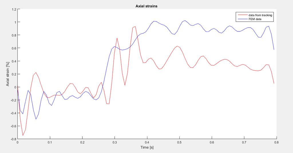
127 NODE 1) 105

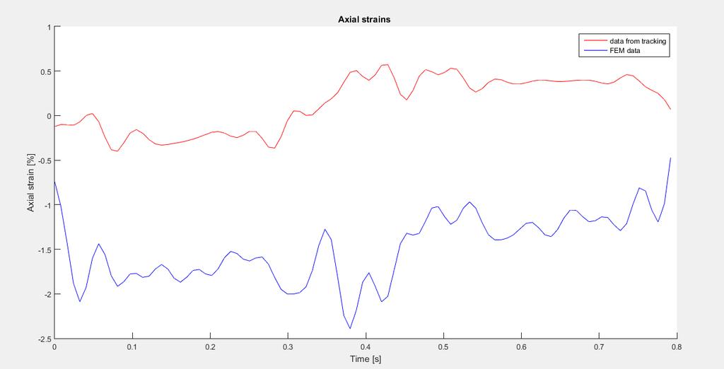
128 NODE 2) 106

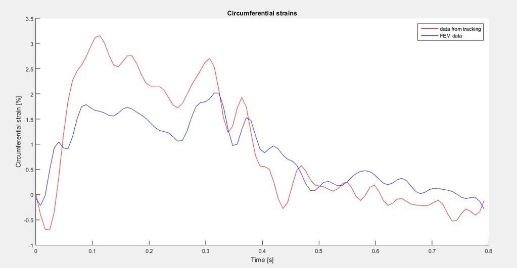
129 NODE 3) 107

130 NODE 4) 108

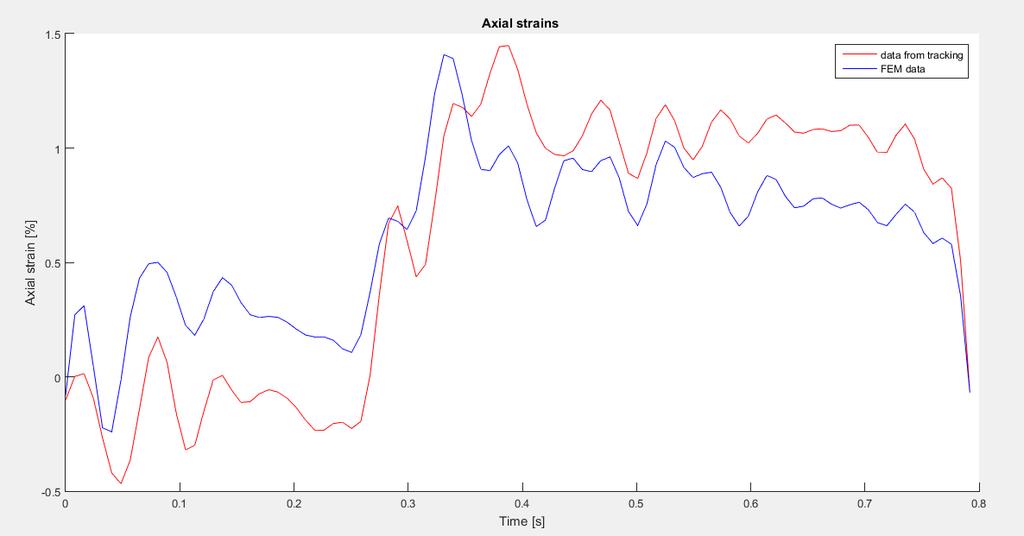
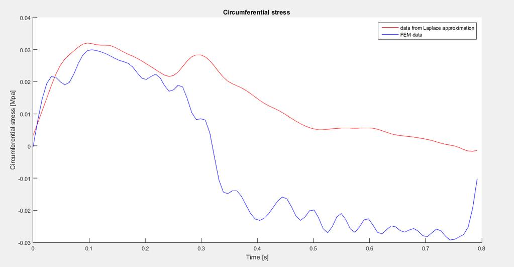
131 109

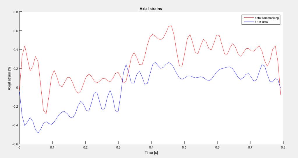
132 NODE 5) 110

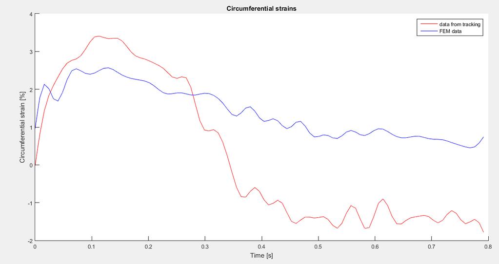
133 NODE 6) 111

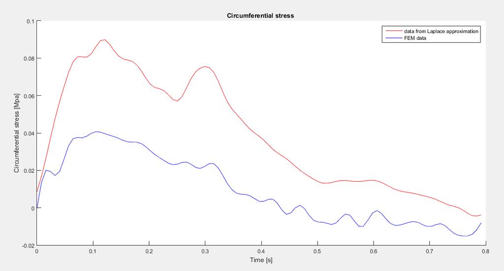
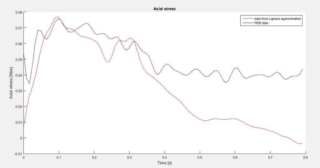
134 NODE 7) 112

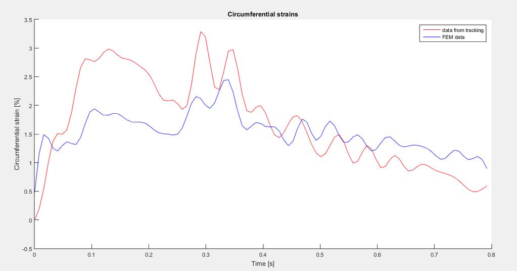
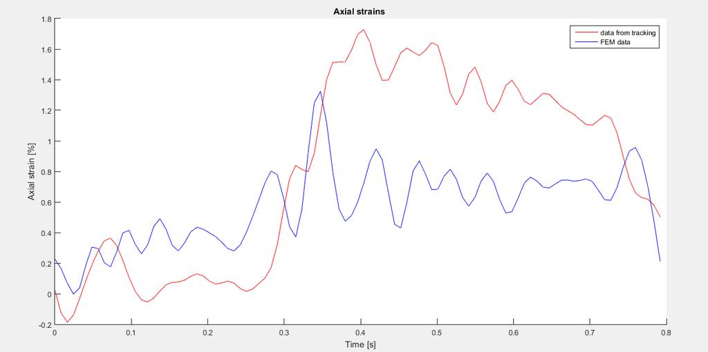
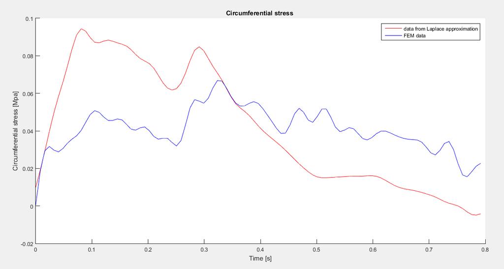
135 113

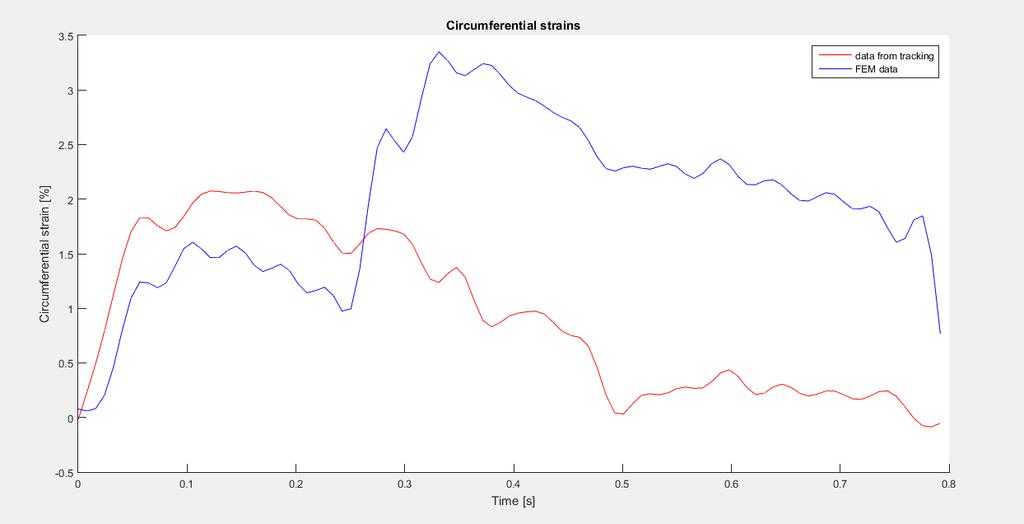
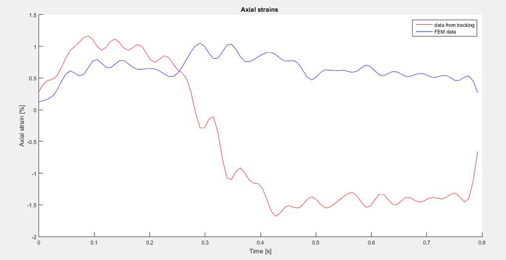
136 NODE 8) 114

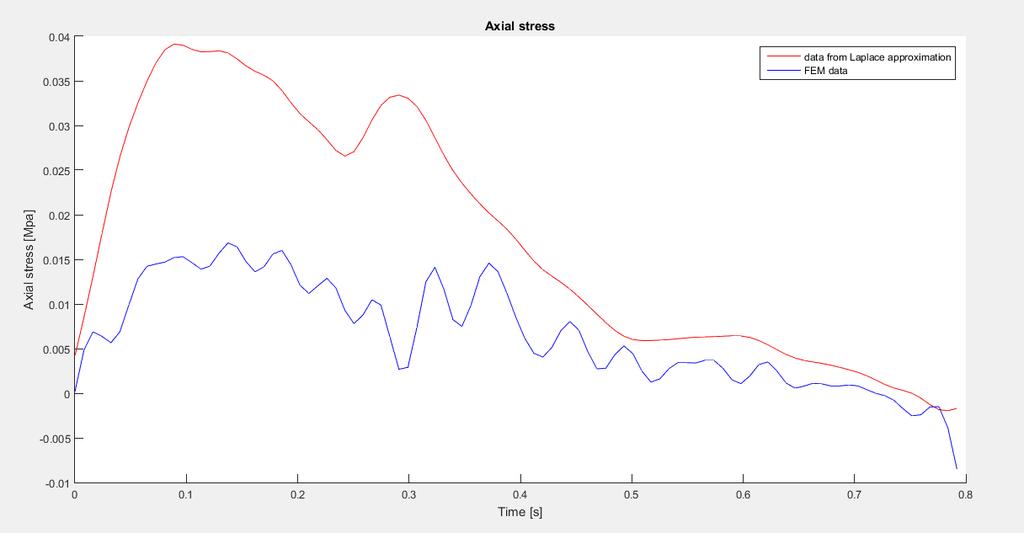
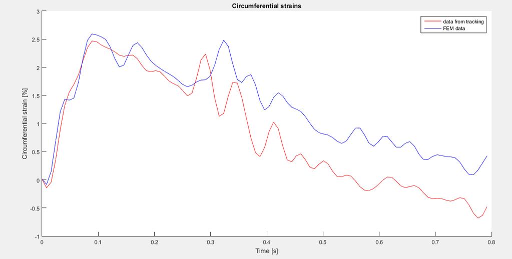
137 NODE 9) 115

138 NODE 10) 116

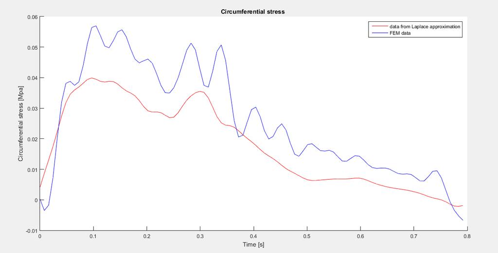
139 117

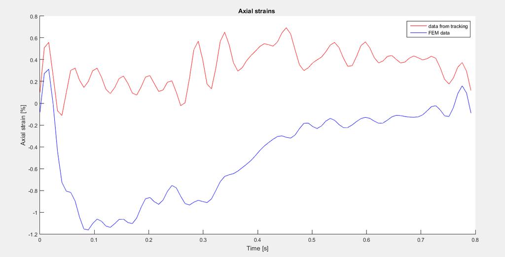
140 NODE 11) 118

141 NODE 12) 119

142 NODE 13) 120

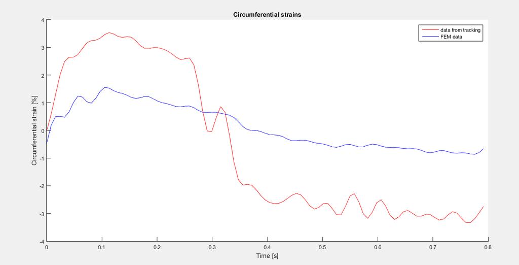
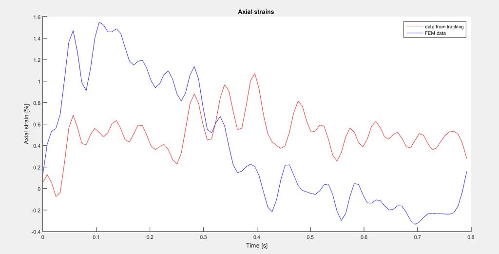
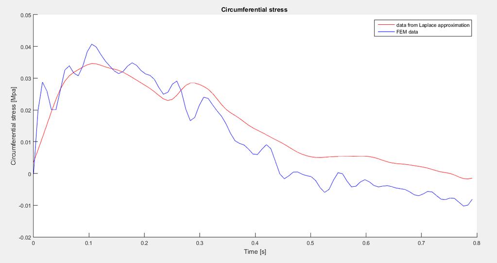
143 121

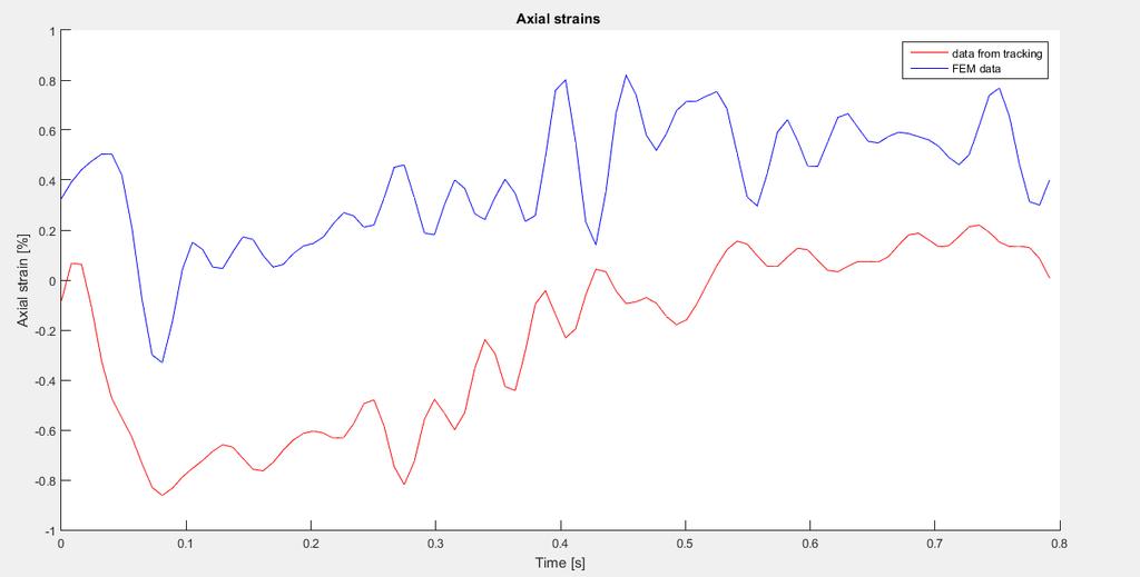
144 NODE 14) 122

145 NODE

146 NODE 16) 124

147 125

148 NODE 17) 126

149 NODE 18) 127

150 NODE 19) 128

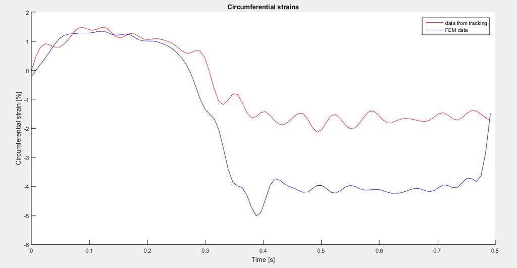
151 129

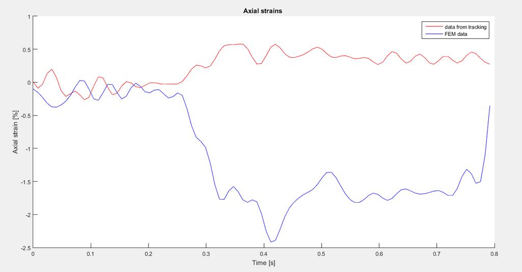
152 NODE 20) 130

153 NODE 21) 131

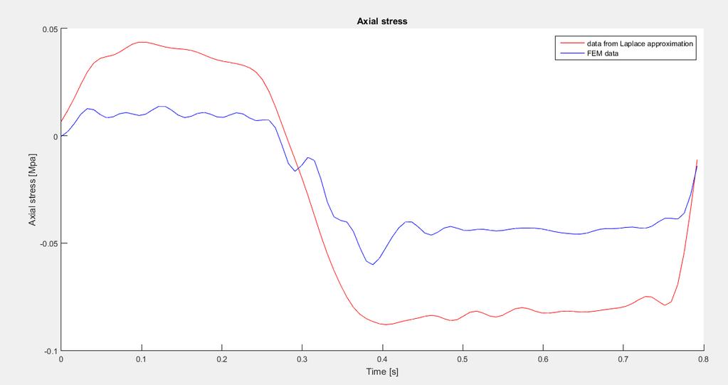
154 NODE 22) 132

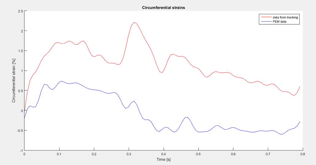
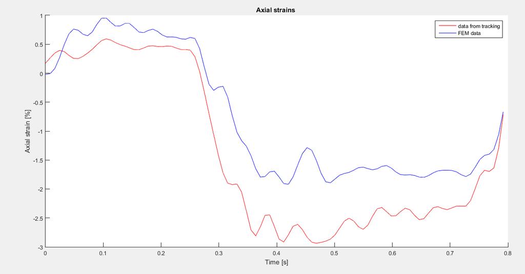
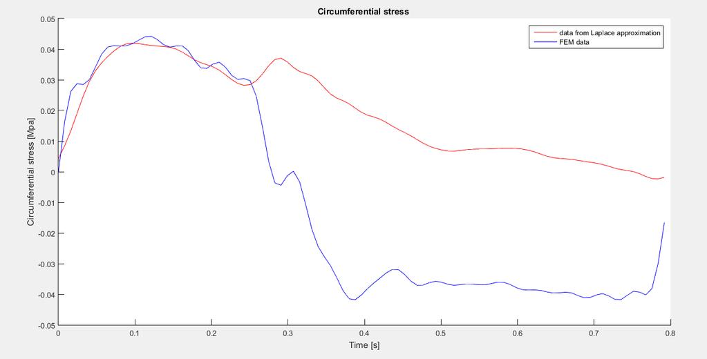
155 133

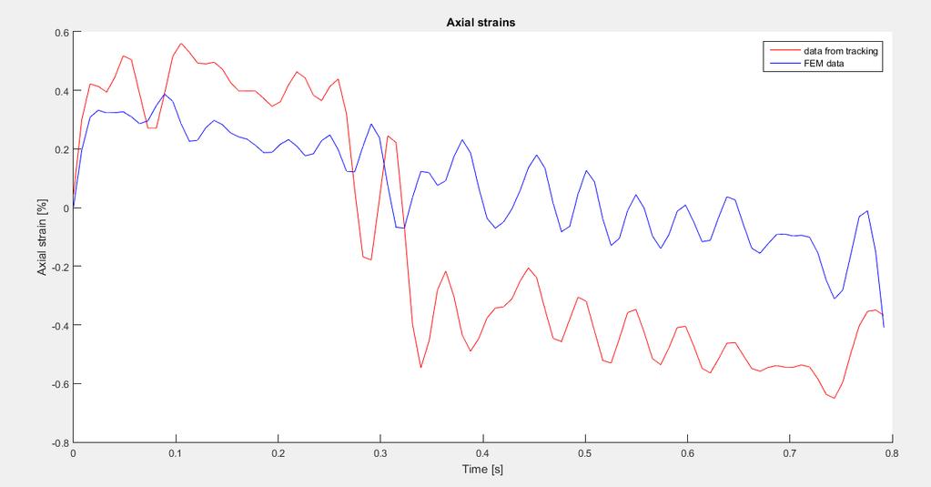
156 NODE 23) 134

157 NODE 24) 135

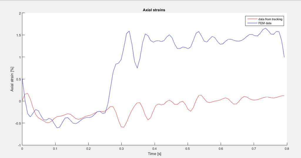
158 136

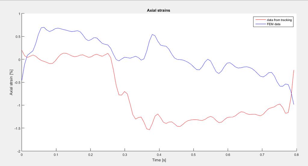
159 NODE 25) 137

160 NODE 26) 138

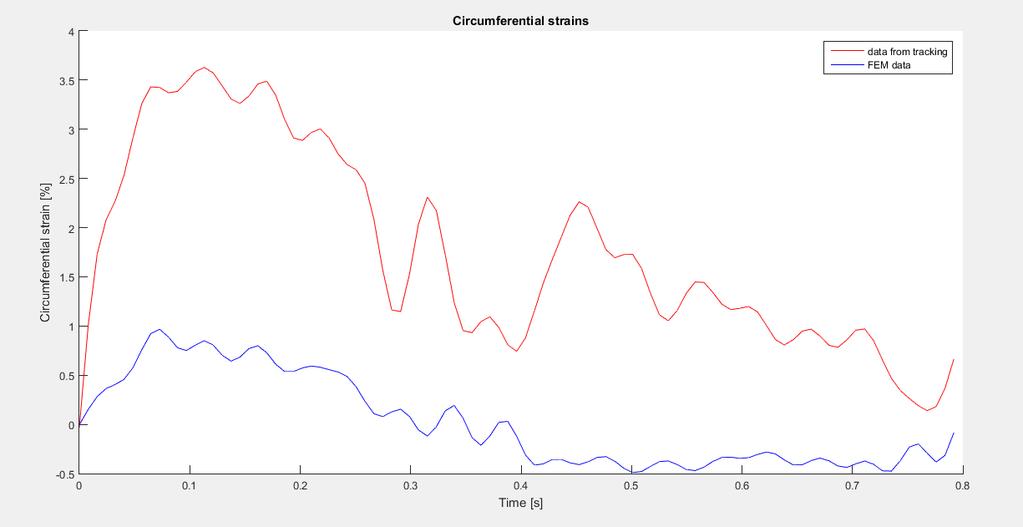
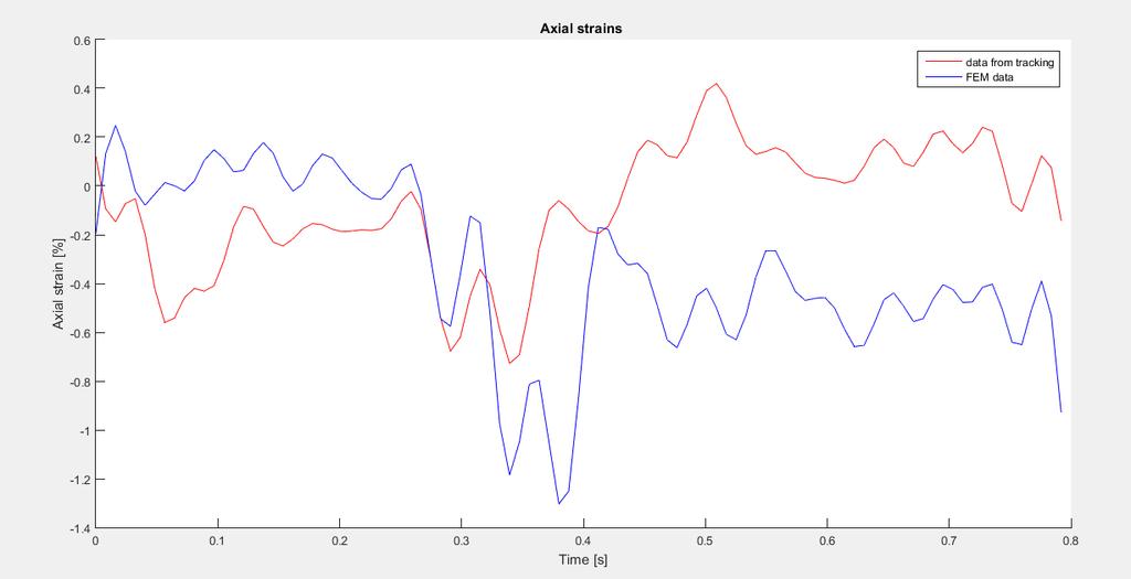
161 139

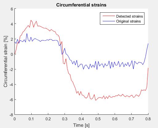
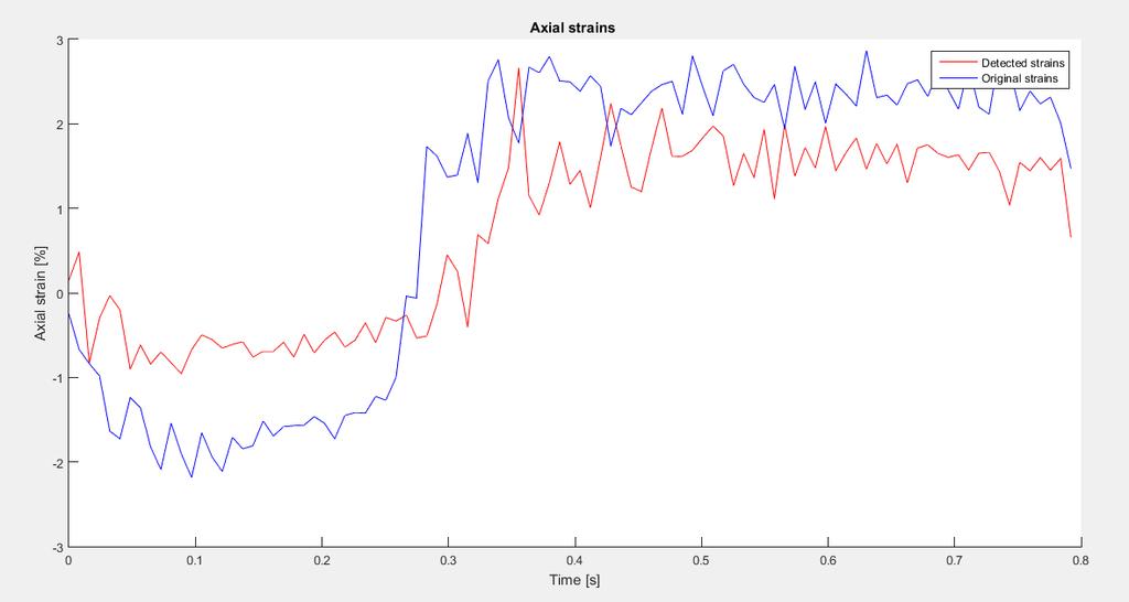
162 NODE 27) 140

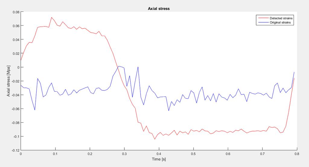
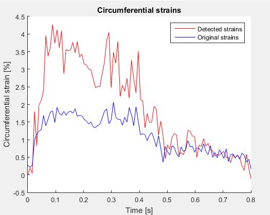
163 NODE 28) 141

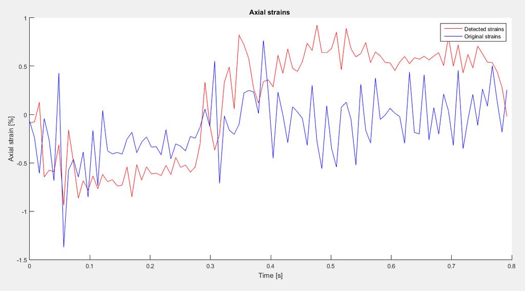
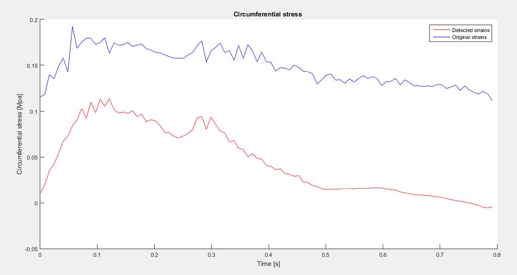
164 142

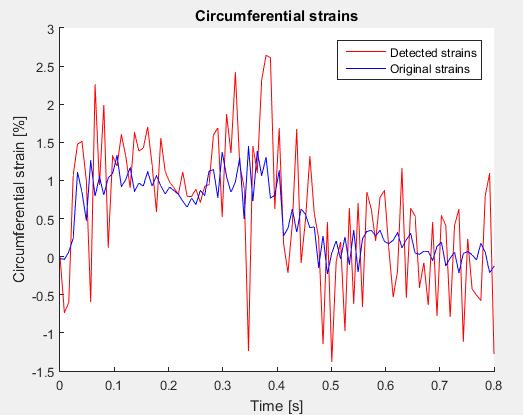
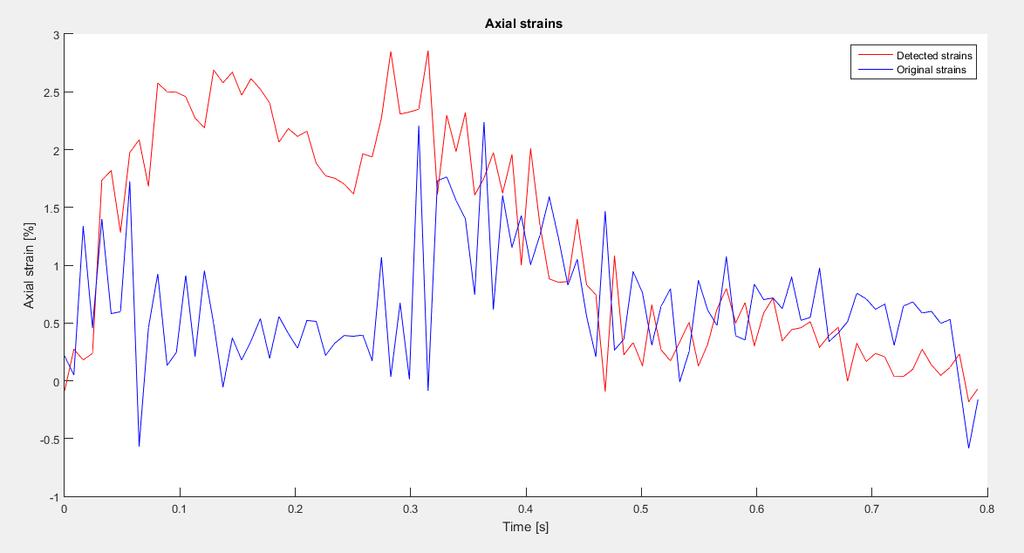
165 NODE 29) 143

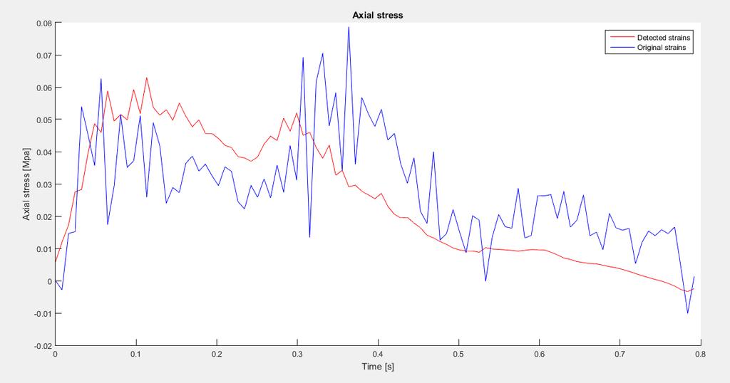
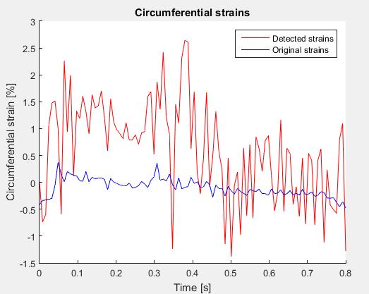
166 NODE 30) 144

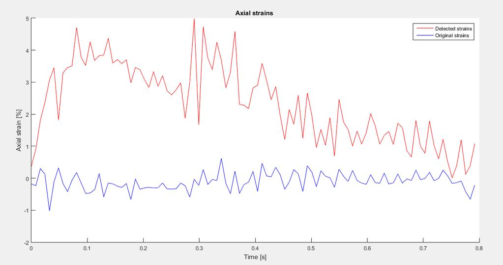
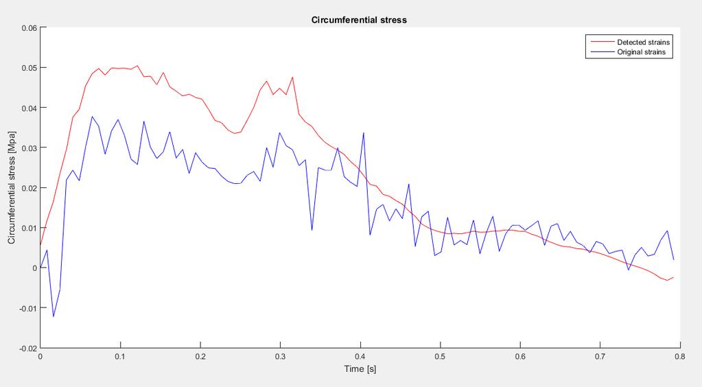
167 145

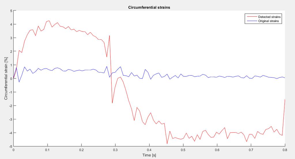
168 NODE 31) 146

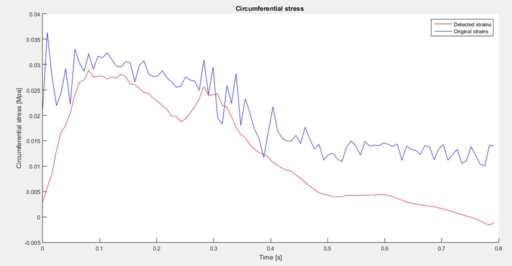
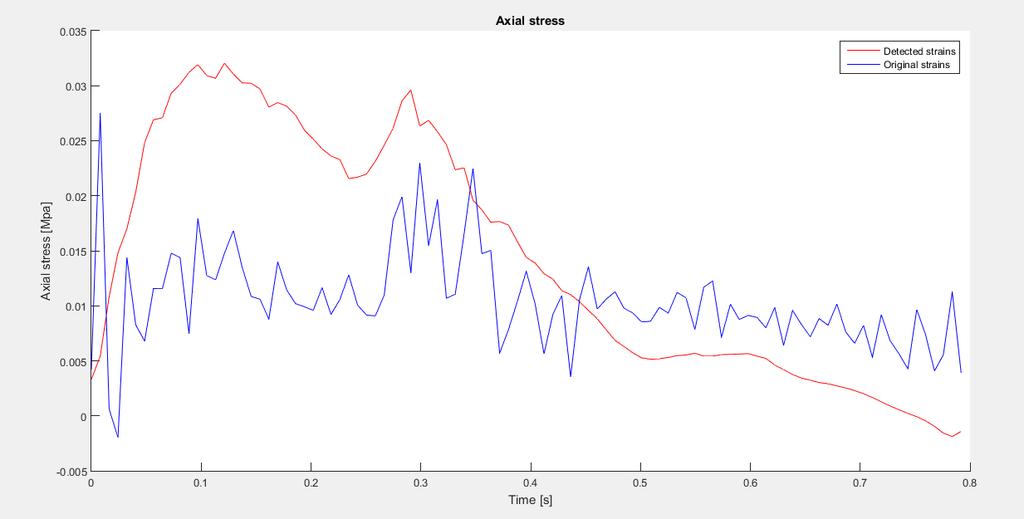
169 NODE 32) 147

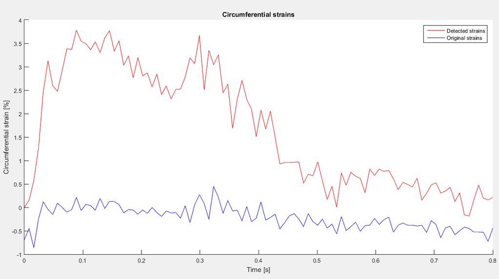
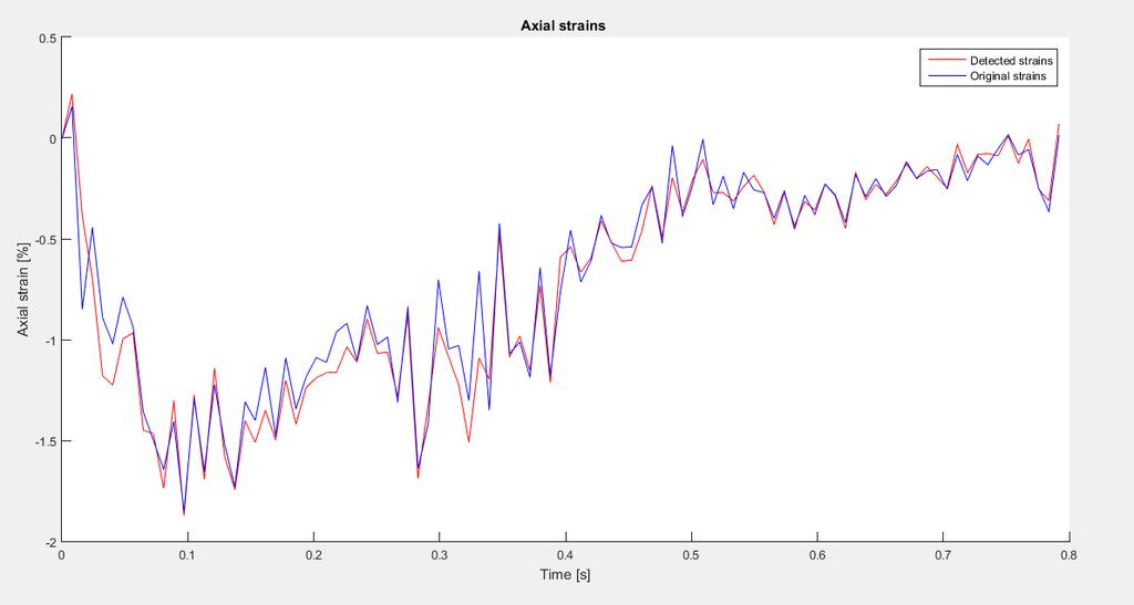
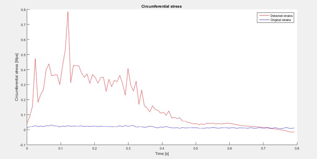
170 148

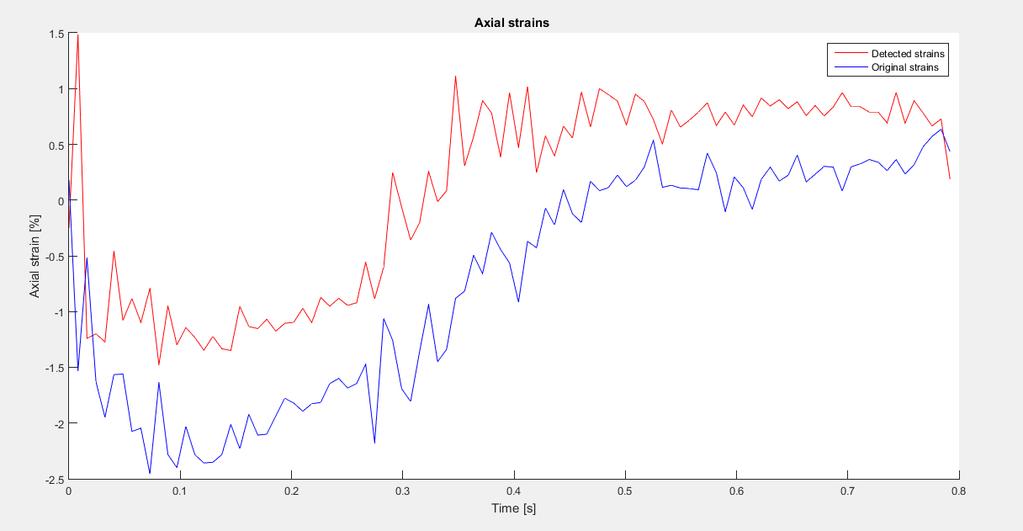
171 NODE 33) 149

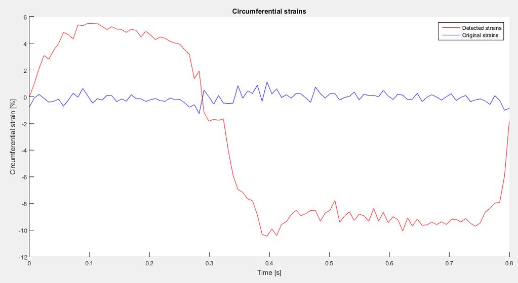
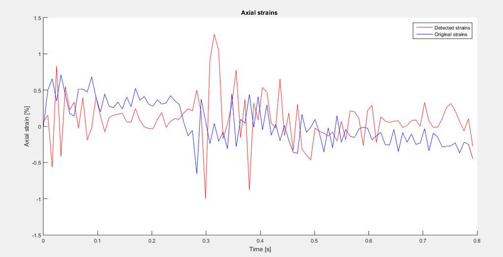
172 NODE 34) 150

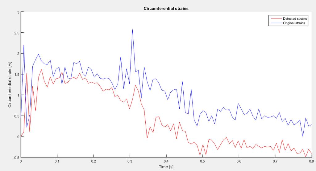
173 NODE 35) 151

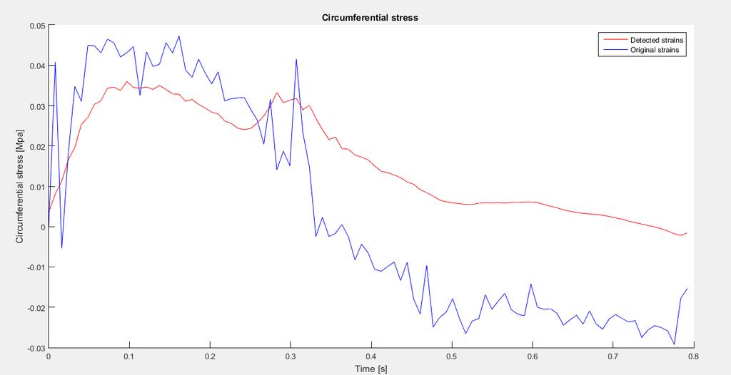
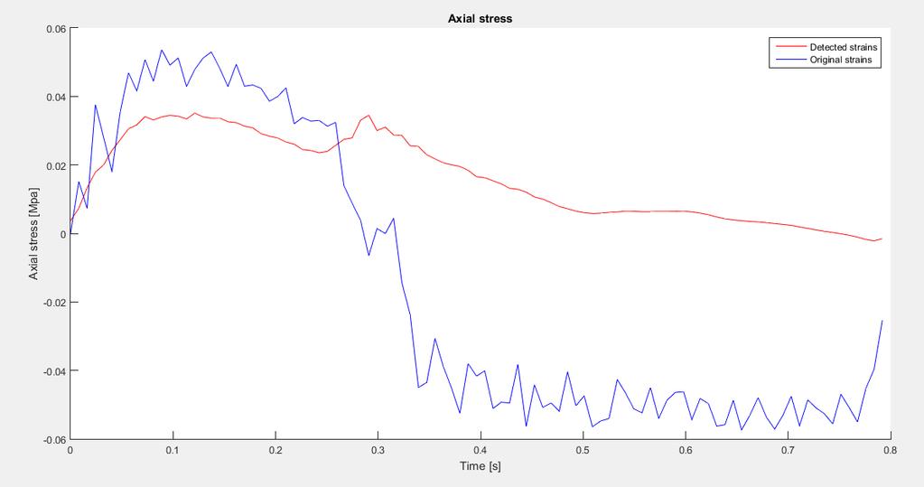
174 NODE 36) 152

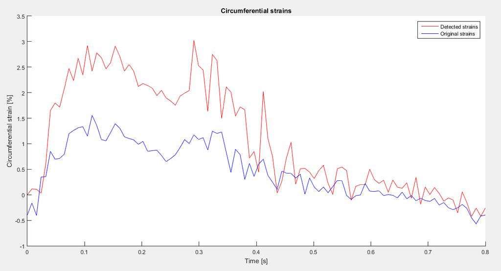
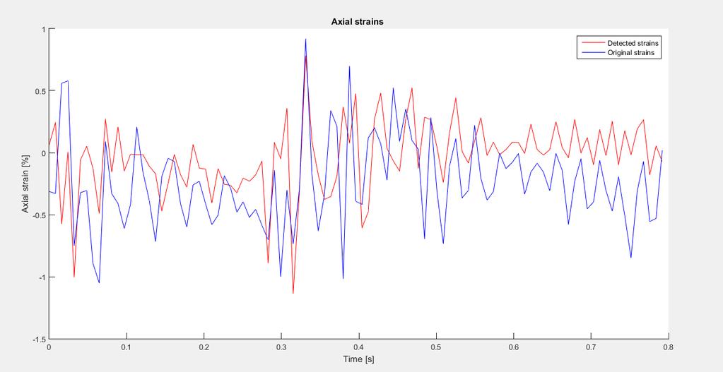
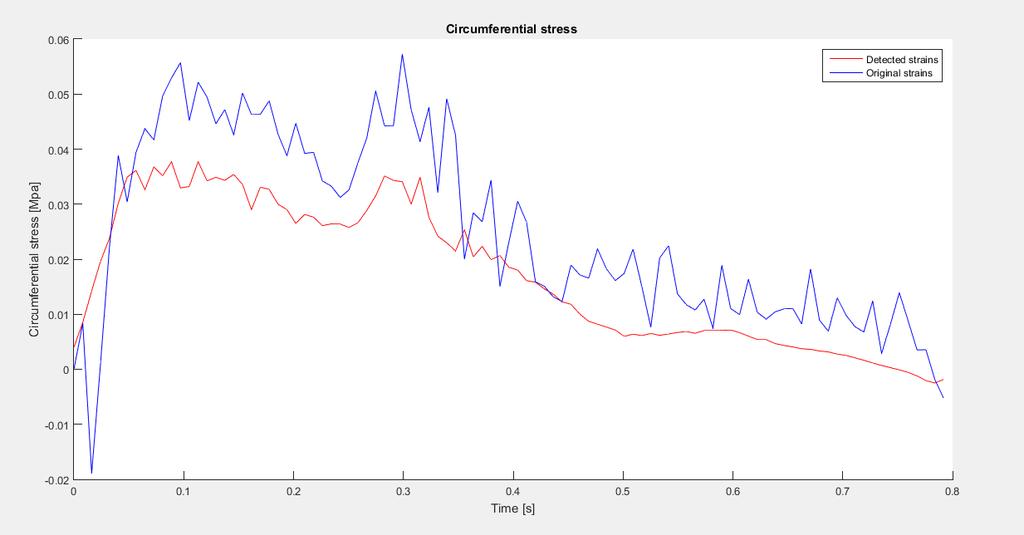
175 153

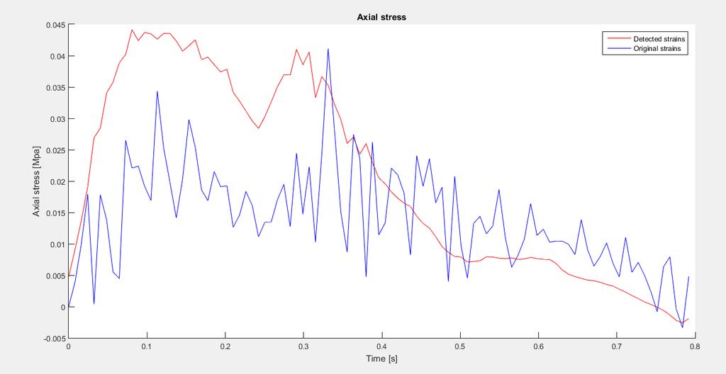
176 154