Real-World Wayfinding Experiments

Transcription

1 Real-World Wayfinding Experiments Individual Preferences, Decisions and the Space Syntax Approach at Street Corners Beatrix Emo University College London a thesis submitted for the degree of doctor of philosophy at university college london 2014

2

3 del bello intelligibile

4 Real-World Wayfinding Experiments Beatrix Emo Bartlett School of Architecture, University College London Doctor of Philosophy in Architecture 2014 Supervision: Alan Penn (University College London) Beau R. Lotto (University College London) Ruth Conroy Dalton (University of Northumbria) Alasdair Turner (University College London) i

5 I, Beatrix Emo, confirm that the work presented in this thesis is my own. Where information has been derived from other sources, I confirm that this has been indicated in the thesis. ii

6 Abstract This thesis investigates the role of spatial configuration on individual spatial decision-making. Over 100 participants take part in laboratory wayfinding experiments based on real-world images of street corners, using fixed and mobile eye trackers. Participants are asked to perform directed and undirected spatial tasks; stimulus-derived and task-related viewing patterns are accounted for. Responses to the spatial tasks are tested for task-related bias against responses in non-spatial tasks (recall, free viewing, and controlled search). The evidence reveals that, during wayfinding, participants choose the more connected street, measurable with space syntax variables of relative street connectivity. Four space syntax variables are used: integration and choice at global and local scales. The resulting measure allows decisions made by individuals to be related directly to the space syntax analysis of spatial morphology. The fixation data allows for an investigation of how wayfinding choices and gaze bias may be linked. Viewing behaviour during the spatial tasks reveals areas of particular interest at each path alternative; these correspond to structural information in the built environment. A measure for identifying the location of such areas is proposed: choice zones. Choice zones are computed algorithmically, and are based on space-geometric measures visible in the scene. Choice zones o er a greater scope than existing measures because they are based on information visible in the real world; itisthereforepossibletocomputechoicezonesforimagesof di erent reference classes (eg. those with varying horizon or sky lines). The resulting measure has important implications for optimal routing and urban design, identifying those areas of the visual field that contain the most relevant environmental information pertaining to wayfinding.

7 Acknowledgements My thanks go to Ruth Conroy Dalton, for sharing her passion and inspiring me to embark upon the PhD. She has been an excellent supervisor, and a constant source of motivation. I am indebted to her for her unfailing support and her feedback on work over the last few years. The late Alasdair Turner was an inspirational tutor and supervisor. I am especially grateful to him for encouraging me to explore the world of eye tracking. Alan Penn has been an outstanding supervisor, coaching me through the many stages of the PhD. It has been a privilege to be supervised by him and I thank him for his valuable comments on my work. It has been very stimulating to be part of Beau Lotto s visual perception lab, and I am especially grateful for the opportunity to run my experiments at the Lottolab Studio, when it was based at the Science Museum in London. My thanks also to Muki Haklay, for allowing me to borrow both eye trackers. This work would not have been possible without the generous EPSRC Studentship. Finally, I would like to thank all of my previous teachers and my parents. Ialonebearresponsibilityforallremainingerrors. iv

8 Publications Some of the material in this thesis has been, or is in the process of being, published in the form of the following papers: (1) Emo, B. (2010). The visual properties of spatial configuration. In Dara- Abrams, D., Hölscher, C., Dalton, R. C., & Turner, A. (Eds.), Environmental Modeling: Using Space Syntax in Spatial Cognition Research, Proceedings of the workshop at Spatial Cognition 2010, Mt. Hood, Oregon, SFB/TR 8 Report No /2010. (2) Emo, B., Hölscher, C., Wiener, J. & Dalton, R. C. (2012). Wayfinding and Spatial Configuration: Evidence from Street Corners. In Greene, M., Reyes, J. and Castro, A. (Eds.), Proceedings of the Eighth International Space Syntax Symposium, Santiago de Chile, PUC. (3) Emo, B. (2012). Wayfinding in real cities: experiments at street corners. In Stachniss, C., Schill, K. & Uttal, D. (Eds.), Spatial Cognition 2012, LNAI (4) Emo, B. (2012). Experiencing the Built Environment through Legibility. In Seifert, G., Planck, C., Zisch, F. & Gschwendtner, G. (Eds.), Proceedings of Spatial Thinking 2, Innsbruck, Austria. (5) Emo, B. (2013). Choice zones: spatial geometry and real world wayfinding. In Kiefer, P., Giannopoulos, I., Raubal, M. & Hegarty, M. (Eds.), Proceedings of the First International Eye Tracking for Spatial Research workshop. Held at COSIT 13, Scarborough, UK. (6) Emo, B. & Dalton, R. C. (2013). Wayfinding and spatial configuration: pedestrian behaviour at street corners. In Kim, Y. O., Park, H. T., & Seo, K. W. (Eds.), Proceedings of the Ninth International Space Syntax Symposium, Seoul,SouthKorea. In particular, material from 1 is in part of chapter 3, part of 2 is in part of chapter 4, part of 3 is in part of chapter 5, part of 5 is in part of chapter 6, and parts of 4 and 6 are in part of chapter 7. v

9 Contents Table of Contents vi List of Figures vii List of Tables viii 1 Introduction Motivation Key concepts Research questions Chapter outline summary Contribution to knowledge Relevant literature Spatial cognition and visual perception during wayfinding Wayfinding Spatial cognition during wayfinding: cognitive maps Visual perception during wayfinding Analysing the spatial structure of the environment Space syntax measures Viewshed analysis Eye tracking as a methodology Eye movements Visual attention Eye trackers Methods Stimulus set Choosing the locations Variety within the stimulus set Creating the stimuli Manipulating the stimuli The stimulus set Supplementary stimuli for the recall task Tasks Spatial tasks Non-spatial tasks Apparatus Desktop-based eye tracker Mobile eye tracker vi

10 3.4 Procedure Spatial and recall tasks Free viewing and controlled search tasks Analytic methods Behavioural data Eye tracking data Analysis without eye tracking Introduction Hypotheses Methods Stimuli Tasks Participants Analysis Results Responses Response times Discussion Analysis with eye tracking Introduction Hypotheses Methods Stimuli Tasks Participants Analysis Results Behavioural choices Response times Eye tracking data Discussion Choice zones Introduction Areas of Interest Space-geometric measures Identification of choice zones Outline of the choice zone algorithm Stepwise definition - details Example choice zones Accounting for the gaze bias Discussion Discussion and conclusion Introduction vii

11 7.2 The role of spatial configuration on wayfinding decisions The role of spatial configuration on gaze bias patterns during wayfinding Implications for how individuals process the axial map Conclusions and future directions References 161 A Segment maps 175 B Stimulus set 179 C Path connectivity in the stimulus set 195 D Questionnaires 199 E Fixation data - spatial tasks 203 F Fixation density distributions according to spatial task 219 G Fixation density distributions comparing the recall and spatial tasks 235 H Defining AOIs - clustering in the fixation data 247 viii

12 List of Figures 1.1 Illustrating spatial configuration Example stimulus Analysing the street network as a graph Angular weighting for segment angular analysis Axial map Segment map Example saliency map E-spaces Junction types Manfrotto panoramic head Example stimulus for the control of light conditions Non-mirrored and mirrored versions of a stimulus Eye trackers Example screenshot of the video data Identifying focus areas for the coding of the video data Example fixation distribution Example gaze bias with accompanying fixation density graphs Comparison of gaze bias undirected & directed spatial tasks Comparison of gaze bias between the recall and spatial tasks AOIs defined arbitrarily Example of AOI-shapes influenced by the gaze bias Fixation clustering at areas of high spatial interest Space-geometric measures Floor line segments Longest line of sight: x-axis values Longest lines of sight: based on floor line segments LLS and the first floor line segment Simplified LLS definitions, when LLS-LLS4 are unique Simplified LLS definitions, when LLS-LLS3 are non-unique Choice zones - based on three ellipses Choice zone visualisations Choice zones - first example Choice zones - second example Choice zones - third example ix

13 List of Tables 3.1 Correlation coe cients between the measures of variation in the stimulus set Average number of decisions per participant that choose the same path alternative in non-mirrored and mirrored instances Average number of decisions per participant that choose the more connected street independent of task Distribution of bias in the directed compared to the undirected spatial task Average number of decisions per participant that follow attractors Average number of decisions per participant that choose the same path alternative following changes to lighting conditions Average number of positive recall responses per participant Average number of decisions per participant that choose the same path alternative in non-mirrored and mirrored instances Average number of decisions per participant that choose the more connected street independent of task Distribution of bias in the directed compared to the undirected spatial task Average number of decisions per participant that follow attractors Average number of decisions per participant that choose the same path alternative following changes to lighting conditions Average number of positive recall responses per participant Average number of fixations per participant that follow attractors Average increase of fixations per participant towards the path alternatives with modified lighting conditions Most popular sequences for the free roaming task Most popular sequences in the controlled search task Average number of fixations accounted for by the choice zone measure xi

14

15 Chapter 1 Introduction Chapter summary Adiscussionofthemotivationandkeyconceptsunderlyingthethesisleads to the presentation of the research questions. The main research question asks how individual spatial decision-making is a ected by spatial configuration. Two subquestions are identified: i) How does spatial configuration a ect wayfinding decisions? and ii) How does spatial configuration a ect visual attention during wayfinding? The chapter outlines the thesis experiments and their findings. The chapter ends with a statement of the proposed contribution to knowledge of the thesis. 1

16 1.1 Motivation How do pedestrians decide which way to go in cities? When going to a known destination, one might say that they take the shortest route (Hirtle & Gärling, 1992). There are di erent ways of measuring shortest path and pedestrians tend to act on some notion of shortest path, whether or not that notion may be the most accurate (Golledge, 1995). This thesis considers urban pedestrian navigation in unfamiliar environments. Specifically, it examines individual spatial decision-making at street junctions. When asked which way to go in an unfamiliar city, di erent types of information are useful, such as visual, linguistic and structural information. For example, during business hours people tend to be present in streets where there are also shops. Thus a pedestrian looking for a shop in an unfamiliar city is likely to choose to go in the direction of crowds of people if these are visible. Signposts, community maps of the area and street names all provide evidence that can help pedestrians find their way. Another type of information, structural information, is also important; this thesis arises out of a body of research that emphasises the relative importance of structural information on pedestrian navigation. Structural information relates to how the building blocks are positioned in relation to the street; it does not relate to photographic or textual elements. One type of structural information that is examined in this thesis is spatial configuration (refer to the definition in section 1.2). Designers tend to work from plans, which are presented at all stages of the design process. Eventually however the building or, more relevant for the purposes of this thesis, 1 the urban area is established, and users of that space begin to populate it. Their experience of the space is refined according to how, 1 The thesis concentrates on navigation in urban environments. Much of the research that discusses urban pedestrian navigation also holds true for indoor navigation, although that is not the focus here. 2

17 and how often, they frequent it, and di erent responses are recorded. In areas where people often feel unsafe or get lost easily, it may be the case that spatial factors play a role (for evidence relating crime hotspots to spatial factors see for example Hillier (2004)). This thesis argues that structural information in the environment accounts for an important part of the individual s experience of the built environment. Several studies o er some insight into the role of spatial configuration on pedestrian navigation (eg. R. C. Dalton (2003), Penn (2003), Hölscher, Brösamle, and Vrachliotis (2012) and Wiener, Hölscher, Büchner, and Konieczny (2012)), although to date very few, if any, have collected empirical evidence of real world pedestrian navigation at the individual level. Space syntax methods offer a way of measuring spatial configuration; however, while the role of spatial configuration on aggregate pedestrian flow has been extensively tested, the role of spatial configuration on individual spatial decision-making needs to be defined. One aim of this introductory chapter is to present the research questions of the thesis (see section 1.3). Prior to that, a number of key concepts are introduced and defined, as they will be referred to throughout the thesis. The relevant concepts that make up the following section are: navigation and wayfinding; spatial configuration; and space syntax. 1.2 Key concepts Navigation can be thought of as an activity of two distinct stages (Montello, 2001). One is locomotion, which refers to the physical act of moving through space; the other is wayfinding, which refers to the act of making decisions. Both parts are equally important, and pedestrians navigating through cities 3

18 use both alike, however it is the decision-making process that this thesis analyses. Wayfinding is defined in this thesis as the decision-making stage of navigation (following the definition of Montello, 2001). A pedestrian approaching a street corner is forced to make a choice as to which way to go, and having made that choice, will continue along that chosen path. Several factors influence that choice, such as the destination, previous experience, spatial ability and personal preference. Many of these parameters have been identified and measured in existing studies (see section for a review). Another factor that is eminently relevant to individual spatial decision-making is the structure of the space which is being navigated. This factor becomes especially relevant when the subject is not navigating to somewhere they have been before. Pedestrians, when making their way to an unknown destination in an unfamiliar area, may rely on clues derived from the structural properties of the environment. The relevance of structural information for human navigation was first highlighted by Kevin Lynch in his seminal study (1960), and further pioneering research was conducted by Jerry Weisman some decades later (1981) (see section for more detail). The proposition resulting from these early research initiatives is that humans draw on information on how paths in a city are linked. This notion is called spatial configuration. Spatial configuration is defined as the way the relationship between any two spaces is altered by their connection to a third space (following the definition of Hillier, 1996; see fig. 1.1). Consider a simple spatial layout where two spaces a and b (eg. rooms) are connected to an outside space c (eg. an entrance). In the first instance, let spaces a and b be connected directly to space c. In the second instance, let the connection b-c be closed o, so that only space a connects directly to space c. It is clear that the relationship of space c to spaces a and b changes the relationship between the three spaces. One could 4

19 Figure 1.1: Illustrating spatial configuration. Image after Hillier (1996) say that the configuration of space has changed significantly from the left to the right hand image. This concept is easily grasped by comparing the graphical representations of the two instances, in which the spaces are depicted as nodes and the connections between the spaces as links. Space syntax o ers a way of measuring spatial configuration that has proved to be a useful tool for practitioners. 2 Acommonspacesyntaxmethodrepresents an environment (indoor or outdoor) as a network of nodes and interconnecting links, which can then be analysed as a graph. Analyses of urban environments have mostly been focussed on the layout of the street grid (rather than on three-dimensional representations); in space syntax research the street grid is often represented as the longest and fewest set of lines completing the network. In simple terms, every straight road on a map of a city is translated into a single line, so that the resulting map is formed solely of a network of interconnecting lines. How exactly these maps are created, and whether they can or should in fact be generated algorithmically, has been debated (see Batty and Rana 2 The description of space syntax methods given here is intended as an overview. For a more detailed discussion refer to section

20 (2004); Turner, Penn, and Hillier (2005)). The resultant map is analysed as agraph;centralityandbetweenessmeasureshaveprovedtobeaparticularly e ective proxy for aggregate pedestrian movement when compared with direct observational counts. Essentially, the space syntax analytical framework o ers awayofanalysingstreetconnectivitythathasbeenshowntorelate,witha high degree of accuracy, to aggregate pedestrian flow. Some of the main findings on the social use of space arising from space syntax analyses relate to the distribution of land use (Hillier, 1996), the location of crime hot-spots (Hillier, 2004), and the distribution of socio-economic town centres (Gri ths, Jones, Vaughan, & Haklay, 2010). 3 These findings are related to aggregate pedestrian flow, although it has been suggested that the nature of the analysis may also relate to decisions made by individuals (Penn, 2003). The lack of evidence relating to this question is a major limitation of the space syntax approach; this thesis addresses this gap in knowledge by applying space syntax measures to data collected from individuals. The approach adopted in this thesis is therefore egocentric. This is in contrast to existing space syntax approaches which are allocentric: space syntax values of spatial configuration are the same all along a segment. Thus by examining the relevance of space syntax measures on the decisions made by individuals, the thesis touches on a deeper philosophical issue regarding the ego and allocentric relationship between viewpoints. 1.3 Research questions The principal research question which this thesis addresses is: How is individual spatial decision-making a ected by spatial configuration? It has been shown that aggregate pedestrian flow is a ected by spatial configuration; how 3 More detail on these examples is also given in section

21 is this reflected in decisions made by individuals? This overarching question is approached through two subquestions. 1. How does spatial configuration a ect wayfinding decisions? This can be tested by examining whether or not the choices made by individuals during wayfinding favour the more connected street How does spatial configuration a ect visual attention during wayfinding? This is tested by analysing the viewing behaviour during wayfinding; in particular, any influence of the spatial geometry of the scene is examined. These research questions are approached through the experiments and analysis in the following chapters. Through the review of concepts in chapter 2, the relevant hypotheses addressing the research questions are reached. Chapters 4, 5, and 6 provide evidence relating to the research questions; this is done by testing several distinct hypotheses, which cover the variable and control factors. Chapter 7 discusses the research questions in light of the findings. 1.4 Chapter outline summary The thesis has eight chapters. Each chapter begins with a chapter summary and ends with the key points to be taken from the chapter. The research questions are presented in the opening chapter, which is intended as an overview to the thesis a whole. Some key concepts are introduced and defined, using non-specific language: navigation and wayfinding; spatial configuration; and space syntax. The chapter ends with the proposed contributions to knowledge of the thesis. 4 The more connected street measure is defined in section

22 Adiscussionofrelevantconcepts,spanninganumberofacademicdisciplines (eg. architectural research, environmental psychology, cognitive science, visual perception), is given in chapter 2. Existing findings are discussed and gaps of knowledge highlighted. The discussion is grouped into three broad areas: i) spatial cognition and visual perception during wayfinding, ii) methods for analysing the spatial structure of the environment, and iii) eye tracking as amethodology. Thechapterprovidesthebackgroundfortheformulationof hypotheses in chapters 4 and 5. Apreciseaccountofthemethodsusedinthethesisisgiveninchapter3. The stimulus set is described in detail. This is followed by a discussion of the chosen tasks. Technical details of the apparatus are given, as well as a full account of the procedural set up of the experiments. The chapter goes on to discuss the analytical methods used, including the measure of the more connected street. Chapter 4 presents behavioural data from subjects choosing which way to go in a wayfinding experiment. 20 participants take part in a binary choice experiment. The experiment set up is described; the data is presented and analysed. Results show that subjects tend to choose the more connected street. A subsequent study explores these decisions from a visual perception standpoint (chapter 5). Eye tracking data records where participants fixate while making wayfinding decisions. The hypothesis that visual attention is drawn to aspects of the spatial geometry of the scene is tested. Control conditions account for the influence of stimulus-derived and task-dependant viewing behaviour. Two eye trackers are used, targeting di erent research questions. More than 100 participants provide a large dataset. The experimental set up is described, reflecting the use of one desktop-based and one mobile eye tracker. The data is presented and analysed. Results from the behavioural 8

23 data confirm that participants tend to choose the more connected path alternative. Results from the eye tracking data show how gaze bias and wayfinding decisions are linked; of particular interest is the viewing pattern during the spatial tasks. The fixation data during the spatial tasks is analysed in relation to the spatial geometry of the scene in chapter 6. A measure, termed choice zones is proposed. The concept is described in detail and an algorithmic definition is o ered. Three space-geometric measures are used in the identification of choice zones; these are defined mathematically. Example images show how the measure can be applied. The chapter ends with a discussion of the potential of the measure. The research questions are elucidated by the results in chapter 7. The findings are discussed in relation to previous research. The merit of adopting an egocentric approach when examining how spatial configuration a ects individual spatial decision-making is evaluated. The chapter considers the possible implications for our understanding of the axial map. The final section evaluates the contributions and limitations of the findings, and proposes avenues for future research. The chapter concludes by assessing the relevance of the thesis for space syntax and spatial cognition research. 1.5 Contribution to knowledge The thesis o ers several contributions to knowledge. Methodologically, it proposes a way of applying space syntax measures onto data drawn from individuals during wayfinding. It does this by assessing whether or not people choose the more connected street. 9

24 Results from the behavioural data contribute to both space syntax and spatial cognition research, as it is shown that participants tend to choose the more connected street. Gaze bias data further contributes to spatial cognition research, by providing evidence of the relevance of spatial geometry during real world pedestrian navigation. To the author s knowledge, no studies to date have achieved this result in real world studies. Acrucialcontributionofthethesisisthepresentationofthechoicezones measure. Space-geometric parameters are used in the identification of choice zones, which are computed algorithmically. The measure provides a way of selecting context-dependant information relevant to wayfinding that can be applied in a variety of situations. Key points of chapter 1 The main research question which the thesis addresses is: How is individual spatial decision-making a ected by spatial configuration? This is addressed through two subquestions: i) How does spatial configuration a ect wayfinding decisions? and ii) How does spatial configuration a ect visual attention during wayfinding? Key concepts, such as navigation and wayfinding, spatial configuration, and space syntax, are introduced and defined. An overview of the the experiments and their findings is given. The proposed contributions to knowledge of the thesis are highlighted. 10

25 Chapter 2 Relevant literature Chapter summary The chapter positions the thesis in relation to existing research. The literature of a number of pertinent issues, spanning di erent academic fields, is reviewed. Three broad areas are discussed: i) spatial cognition and visual perception during wayfinding; ii) methods for analysing the spatial structure of the environment; and iii) eye tracking as a methodology. Previous methodologies are evaluated and the reasons for opting for the chosen methods (presented in the subsequent chapter) are given. 11

26 This chapter provides a theoretical background to the thesis by reviewing the body of relevant literature across several fields. The discussion is grouped into three sections: i) spatial cognition and visual perception during wayfinding; ii) methods for analysing the spatial structure of the environment; and iii) eye tracking as a methodology. 2.1 Spatial cognition and visual perception during wayfinding This section discusses the factors that a ect wayfinding, and the cognitive and perceptive processes at work during individual spatial decision-making. It begins by discussing di erent definitions of the term wayfinding Wayfinding Several factors that can be held to a ect wayfinding behaviour are evaluated, and the various ways of recording such behaviour are considered, including the merit of a real world compared to a virtual world experiment. Definitions of wayfinding This thesis explores the decision-making stage of navigation, also known as wayfinding (refer to definition in chapter 1). 1 The process of finding one s way depends on a multitude of factors; this is especially true in an urban setting. The etymological roots of navigation come from the Latin navis, whichrefersto the art of travelling, often by sea. While the term wayfinding is not (yet) listed 1 This study limits itself to human wayfinding behaviour; there is a large body of literature on the behaviour of various categories of animals, birds and insects (see for example Bingman, Jechura, and Kahn (2006) on birds and Collett and Collett (2002) on ants). 12

27 in the Oxford English Dictionary, it has close links to other words that appear there: wayfaring is an archaic term that means travelling, and a wayfarer is atravellerbyroad,especiallyonewhotravelsonfoot. Ithasbeensuggested that the word wayfinding also owes its roots to the word pathfinder, coined by J Fenimore Cooper is his novel of the same name (Bovy & Stern, 1990). This connection is strengthened by the fact that the German word pfadfinder closely relates to what we mean by the term wayfinding. The definition of wayfinding used in this thesis refers to cognitive processes that are used to make navigational decisions. There are however a number of alternative definitions. Lynch (1960) refers to way-finding: a consistent use and organisation of definite sensory cues taken from the external environment. Arthur and Passini (1992) o er many definitions in their book, relating to spatial orientation and spatial problem solving. The cognitive element is referred to in definitions by many researchers (eg. Gibson, 1979; Downs & Stea, 1973; Kaplan & Kaplan, 1982; Golledge, 1999). Some definitions specifically evoke the existence of cognitive maps which are discussed in more detail in section (eg. Kitchin & Freundschuh, 2000). These aspects will be discussed. The definition used in this thesis, based on the Montello (2001) definition, identifies wayfinding as the decision-making process of navigation; it refers therefore to individual spatial decision-making. What factors influence wayfinding? Several factors influence wayfinding behaviour. Some relate specifically to the individual, such as whether they are familiar with the environment, the type of spatial knowledge available to them, the nature of their destination and what their spatial abilities are. Other factors relate to the environment itself, such as spatial configuration. The ensuing paragraphs discuss what factors a ect 13

28 wayfinding and how they can be controlled for. Spatial knowledge. Acrucialfactordefiningwayfindingactivitydepends on what level of knowledge the subject holds about the destination location, how to get there, and the intervening locations. These three types of knowledge have been termed landmark, route and survey knowledge (Siegel & White, 1975). Survey knowledge (also frequently compared to map or top-down knowledge) refers to an understanding of the entire area; for example, when standing at a street corner, survey knowledge would inform the subject as to how that street relates to the street grid as a whole. This thesis does not set out to examine the role of survey knowledge on wayfinding behaviour; therefore participants were chosen (for the response tasks) who were unfamiliar with the area of study. Route knowledge is acquired through the sequential act of moving through an environment. 2 This thesis does not aim to contribute to the discussion on the influence of route knowledge during wayfinding, as the locations shown to the participants were not bound to a route, so they were unable to draw on route knowledge. Landmark knowledge refers to the most detailed type of spatial knowledge. Commonly it refers to identifiable elements of a landscape; Lynch (1960) for example analysed the use of physical landmarks in the sketches of his participants. While this may be a common use of the term, landmark knowledge need not refer to something that might be labelled on a tourist s map. An alternative definition has been proposed, that labels the concept destination knowledge (Wiener, Büchner, & Hölscher, 2009); however this definition refers more to the type of task than to a specific type of knowledge (see discussion below). A suitable definition of landmark knowledge relates to any information that can be gained from the observer s standpoint. This definition brings the term far closer to Gibson s concept of a ordances, 2 Note that movement is a critical factor in Gibson s theory of the observer (1979); see section

29 which are elements that hold meaning for the observer (1966). Participants in an unfamiliar setting make choices based on information within the scene. A common type of a ordance are people: it is known that people tend to follow people (see the section below on attractors). In order to disambiguate from Gibson s highly specific term, elements in an urban scene that typically draw people are termed attractors. Attractors are a type of destination knowledge that are specifically controlled for in this study. Familiarity. The amount of previous exposure to an environment is a critical factor a ecting wayfinding. This exposure can take the form of prior physical excursion in the environment, or experience gained through aids such as maps. The role of familiarity on orientation was highlighted by Gärling, Lindberg, and Mantyla (1983). More recently, the e ect of previous experience on wayfinding performance was found to be critical in the type of strategy used in experiments conducted in a complex, multi-level building (Hölscher et al., 2012; Hölscher, Meilinger, Vrachliotis, Brösamle, & Knau, 2006). This thesis discusses wayfinding activity in unfamiliar environments. The e ect of familiarity is controlled for as all participants who made behavioural choices were not familiar with the area of study. Task. The type of destination a ects wayfinding. When going to a friend s house we might make di erent wayfinding choices than when searching for amuseumentrance. Studieswishingtoexaminewayfindingbehaviourmust therefore be acute in their identification of a task. Many previous examples of tasks used in wayfinding studies exist; these have been grouped into a proposed taxonomy of tasks (Wiener et al., 2009). Asimpleinstanceofwayfindingiswhenasubjectisfacedwiththebinary choice of going either one way or another. The outcome of this choice depends 15

30 Figure 2.1: Example stimulus crucially on the implicit or explicit purpose of wayfinding and its context. It follows that the same subject looking at the same scene in two instances, with adi erentpurposeinmindineachcase,mightwellreachadi erentconclusion as to which way to go. For example, if the purpose in viewing image 2.1 is to find a bus, the subject will clearly opt to take the right hand path. This is the logical path choice given that there is a bus at the end of that path. No assessment of how connected each of the path alternatives seem has to be made once it has been recognised that there is a bus in the right hand path alternative. Any attempt to quantify the spatial structure of the urban grid as justification for why the subject would go right would be out of place. Similarly, a subject whose intended purpose when viewing the above scene was to find a private dining club, might consider taking the left path in order to look at the logo on the flag hanging outside one of the buildings. Thus, when an individual is roaming freely, as in the simplest form of wayfinding, it is di cult to assess their wayfinding behaviour without knowing the purpose of their actions. 16

31 The choice of task crucially depends on the type of information available. This study looks at undirected and directed wayfinding, where there is no information relating to route or survey knowledge. Two spatial tasks are introduced in the subsequent studies, an undirected and a directed instance (see section 3.2). A spatial task during wayfinding is one that specifically encourages the use of spatial information for its successful completion. It should be noted that the labelling of these tasks does not entirely suit the definitions proposed in Wiener s taxonomy, because of the assumption in the Wiener model that a lack of destination knowledge can be complete. In this thesis, rather, it is argued that there must surely be an implicit purpose even to undirected wayfinding. Anumberofgoalsmaybeconsideredimpliciteg. exploration/exercise,as well as other, experiential motivators such as avoiding noise or tra c, or even getting mugged: all of these might lead to explicit choices in spite of no point destination being involved. Individual di erences. The role of individual di erences is a major issue in the field (see Allen (1999); Hegarty and Waller (2005); Wolbers and Hegarty (2010)), and the majority of studies aim to control for variation between individuals. A number of di erent tests exist to account for a variety of factors, the most common of which is spatial ability. Some of the more frequently used tests for spatial ability are the Vandenberg Mental Rotation Test (Vandenberg &Kuse,1978)),andthebroaderQuestionnaireonSpatialRepresentation (Pazzaglia & De Beni, 2001). Related tests include the Santa Barbara Sense of Direction test (Hegarty, Richardson, Montello, Lovelace, & Subbiah, 2002), atestforverbalintelligenceusingavocabularytest(eg. Ekstrom,French,and Harman (1976)) and a test for working memory using the Arrow Span Test (Shah & Miyake, 1996). Spatial ability is not specifically tested for in this study, as there is no correct wayfinding choice: participants are free to choose 17

32 either path alternative. It may be the case that further work wishes to examine the spatial ability and personal preference of the individuals. This would be in keeping with a body of research interested in individual di erence during navigation. However, the focus of this thesis is on the role of spatial configuration; restraints in the scope of the thesis meant that, although of potential interest for a complete consideration of individual preference, this was not controlled for. It is however duly noted as an avenue for future research. Environmental variables. Another factor influencing wayfinding is derived from the environment itself (in contrast to those discussed previously, that relate either to the individual or to the action). One type of environmental variable that has been examined refers to structural information. As already defined (refer to chapter 1), a pertinent example of structural information of an environment is spatial configuration. Agrowingbodyofresearchoverthelastdecadeshasprovidedincreasingevidence to suggest that structural information in the environment is important during navigation. Lynch s work The image of the city, inwhichheidentified five elements of the built environment that were present in mental maps, led the field (1960). Weisman s paper directly identified spatial configuration as a relevant factor during wayfinding (1981). A syntactic approach to space, led by Hillier s group at UCL, defined spatial configuration and, crucially, proposed a way of measuring it (refer to Hillier & Hanson, 1984 and Hillier, 1996). A few papers have examined the role of spatial configuration in real situations. An early study suggested a positive influence of spatial configuration on wayfinding performance (Peponis, Zimring, & Choi, 1990); this was substantiated in a later study that examined a large number of participants during wayfinding in hospitals (Haq & Zimring, 2003). The first substantial study testing the role of topological connectivity on individuals revealed relevant patterns in pause 18

33 behaviour (Conroy, 2001); that study was largely conducted in virtual environments. To date, the current research has not been extensively tested at an individual level, nor has it been tested in real world environments: this is one of the aims of this thesis. This study aims to test the role of street connectivity on wayfinding behaviour. This is achieved i) by analysing participants decisions according to space syntax measures of spatial configuration and ii) through the introduction of the taxi rank task, that encourages participants to choose the more connected street (refer to section 3.2 for a discussion of the tasks). Attractors. The presence of attractors has a strong influence on wayfinding activity. Attractors are defined as those elements that skew wayfinding behaviour towards them; common examples are people, vehicles and also light. Previous research has indicated the e ect of some of these factors, notably the presence of people. Zacharias (2001) shows the e ect of various signs of human activity on wayfinding behaviour, especially the presence of other people. Pinelo (2010) shows how behaviour and gaze bias are directed towards di erent forms of attractors such as people and building edges. Light has long been considered an attractor on human movement (see for example Antonakaki (2006) for a study on the social dimension of the e ect of light). Furthermore, the e ect of light as an attractor for viewing behaviour underlies the concept of saliency, whereby visual attention is directed towards areas of special interest (refer to the discussion in section 2.3.2). For a greater discussion of the e ect of attractors on wayfinding behaviour refer to R. C. Dalton, Tro a, Zacharias, and Hölscher (2011). 19

34 Recording wayfinding Anumberofexperimentaldesignsforrecordingwayfindinghavebeenused, and are discussed here. An additional issue is whether to record in the physical environment, or to use some form of representation; this aspect will also be addressed. Experimental set-up. Early experiments designed to record wayfinding behaviour often relied on the participant describing the decision-making process. This could be achieved either in the physical environment, or by showing participants some type of representation (eg. an image) in a more controlled setting (for an example of early wayfinding experiments refer to Passini, 1984). The major disadvantage of this approach is the dependence on the process of verbalisation, which is i) one-step removed from the decision-making process itself, and ii) highly subjective. Developments in the experimental design of wayfinding studies aim to record the decision-making process directly; this can be done in a number of ways. One way is some direct form of assessment in the form of a questionnaire or tests (eg. spatial orientation tests). Although these may seem fairly rudimentary forms of assessment, they are common given their ease of implementation. Another way is to have the decision-making process noted by an observer. This is often the case when a participant is followed, at a distance, and behavioural aspects held to be related to decision-making processes are recorded. The obvious disadvantage of such a technique is the disparity between the participant and the observer. 3 The most common way of examining wayfinding behaviour is to record the decision-making process directly using computers. The participant indicates their decision instantly through a computer; in this 3 Note that these techniques are often coupled with route traces, that record the locomotory stage of navigation (and not the decision-making process). 20

35 manner, the process of verbalisation of the process is removed. Numerous experimental set-ups exist; the most frequent use one or multiple monitors and akeyboard/joystick. Other aspects of human behaviour can also be taken into account when recording wayfinding. An important feature is where we look. The use of eye-tracking techniques in wayfinding studies is becoming more common. Findings from eye movement research propose, in simple terms, that eye movements are an indication of attention, which in turn is related to what we think. 4 Aneurological approach is also possible; a number of functional Magnetic Resonance Imaging (fmri) studies exist to date that examine brain activity during navigation. The availability of fmri scanning techniques to researchers interested in human navigation is a great asset to the field, as they allow the direct examination of brain activity. In addition, participants eye movements can also be recorded during the scanning process, providing additional data. Existing results using these techniques indicate the relevance of the hippocampus. However, whilst technological advances make the use of eye tracking ever more accessible, the high entry cost of fmri techniques renders their use for wayfinding research still limited. In addition, a fmri scanner cannot be taken into the field. Virtual or real world setting. Ideally, wayfinding studies would always be performed in situ; this would ensure that any findings are directly responding to the physical environment of the study. However, recording wayfinding behaviour in the real world poses problems, due to the inability to control for all compounding variables. In real world studies, i) the experiment design cannot be as robust as for laboratory-based experiments, and ii) data collection may be influenced by other factors (eg. noise). A large number of navigationrelated studies are based on experiments conducted in laboratory settings, 4 For more detail on this refer to section

36 using some type of representation of the physical environment. Studies that use artificially-created stimuli are referred to as virtual reality (VR) studies. Various VR methodologies exist, ranging from the simple monitor/keyboard set-up mentioned previously, to immersive techniques, which aim to o er as complete an experience as possible. The nature of the environmental representation varies, from simple black and white sketches to models with full photographic textures. The main advantage of VR studies is the ability to control parameters; it is possible to vary only one variable whilst controlling all others. Thus, any findings can be ascribed to the variation of the tested factor. A debate exists over the merit of VR studies for navigation-related research. While similarities have been shown in some aspects of behaviour when comparing VR and real-world behaviour (R. C. Dalton, 2003), VR studies cannot be considered a substitute for experiments conducted in real world settings. This is because the very nature of a VR setting is a manipulation of how we actually experience the environment. Possibly the most robust form of analysis would include both types of study, although of course such a set-up is costly. This study o ers a compromise by using photographic stimuli in a laboratory setting. The experimental design is still termed real world as opposed to VR, because the stimuli are not artificially-created; however it should be clear that the experiments are not conducted in situ, rather in a laboratory Spatial cognition during wayfinding: cognitive maps The way in which an individual makes spatial decisions in the built environment involves an understanding of how we process the information we receive. The field of spatial cognition, broadly speaking, is concerned with how we act upon decisions (made in here ) based on the information in the environment 22

37 ( out there ). 5 The field considers the cognition of space through a number of interdisciplinary approaches, including for example those common to linguistics and robotics. The discipline spans a vast number of topics, such as spatial perception, spatial memory, cognitive modelling, individual di erences, neuroscience and navigation; a recent book o ers an overview of these topics (Waller & Nadel, 2013). Perhaps the most relevant aspect of spatial cognition for the discussion in this thesis is the research on cognitive maps, to which this section is dedicated. Cognitive maps are mental graphical representations of the environment connected with aspects of brain activity. The pioneering study that coined the term cognitive map resulted from maze experiments with rats, in which it became clear that rats were able to associate their actions with the spatial elements of the maze (Tolman, 1948). An ensuing body of research has provided a great deal of knowledge as to the spatial reference framework used in navigation in clinical and human research (refer to Wang and Spelke (2000, 2002); Wang (2012)). There is a vast body of literature on various aspects of cognitive maps (see for example Downs and Stea (1973); Evans (1980); and Kitchin and Freundschuh (2000)). How a cognitive map is structured is important given that it contains information (spatial, environmental and previously experienced) about the surroundings, including those beyond the immediately visible; Tolman was the first to advocate its map-like qualities (1948). A critical development in our understanding of cognitive mapping came as a result of findings in cognitive neuroscience, and specifically that the part of the brain known as the hippocampus may be tied to the creation and implementation of cognitive maps (O Keefe & Nadel, 1978). Significant advances have been made in this direction (refer to Andersen, Morris, Amaral, Bliss, and O Keefe 5 Note Norman s well-known distinction between knowledge in the head and knowledge in the world (Norman, 1988). 23

38 (2007) for an overview). The properties of various cell types are focus of much research - it would seem that there are three types of cells representing di erent types of spaces: place cells describing where, headdirectioncellsonthedirec- tion, andgridcellsreflectingthedistance. It might even be conceivable that these forms of representation present in brain cells can be matched by architectural analyses of the environment, with place cells measured by topological relations, head cells by angular analyses, and grid cells by metric valuations (R. C. Dalton, Hölscher, & Spiers, 2010). A large number of studies have identified the role of the hippocampus during wayfinding (see for example Hartley, Maguire, Spiers, and Burgess (2003); Spiers and Maguire (2007, 2008)). A number of studies have examined the role of cognitive maps on wayfinding behaviour, notably on how information is ordered and depicted. The role of topological relations is of particular note, as there is evidence to suggest that topological relations underlie both the cognitive element and the space syntax analysis of the environment (eg. (Kim, 1999; Kim & Penn, 2004; Haq, 2003; Mora, 2009)). Another approach tests possible relations of cognitive and axial maps through agent simulations (Turner, 2006). Certainly, more work should be done to clarify the role of the cognitive map on wayfinding, and in particular on any similarities between the topological relations present in cognitive maps (as well as any neuroanatomical basis for this) and in space syntax representations of the environment. While this thesis sheds light on how individuals interpret the axial map, this is not achieved through cognitive maps, and as such they will not be a part of the subsequent analysis; future research may wish to address this. 24

39 2.1.3 Visual perception during wayfinding This section gives an overview of some of the key thoughts on how we process visual information relevant to the field of visual perception (refer also to section on eye movements); refer to Gordon (2004) for a greater discussion of the history of visual perception. One of the most intriguing questions in the field of visual perception is how we perceive a single object as a whole, even though we may have perceived it from numerous standpoints. An important movement in the history of visual perception that addressed this question, was that of the Gestalt psychologists. Key figures, such as Wertheimer, Köhler and Ko a, are known for their research into the perception of form, or Gestalt, a term previously introduced by Ehrenfels (1890). Experiments led them to believe that Gestalt was a product of the relationship between elements; the overall quality of form was seen as greater than the sum of the parts. For them visual perception was an organised process governed by Prägnanz, aqualityofwholenessorsimplicity.theyalso formulated a number of laws of grouping (eg. proximity, symmetry, similarity etc.), certain of which are still being researched for their relevance on visual perception. Despite the relevance of many of their findings, the Gestalt psychologists did not produce a fully-functional model of visual perception. The traditional approach to vision is dominated by the retinal image, the existence of which was first identified in the early findings of Kepler (1604). According to this view, when we perceive an object from di erent vantage points, each viewpoint results in a variation of the retinal image. In fact, there are multiple possible variations, so that the form of a retinal image need not correspond uniquely to any one 3D image in the real world (Heft, 1996). Indeed, there exist a near infinite number of possible sources for any retinal image, so that the process 25

40 of visual perception is actually based on the probability that a retinal image corresponds to any 3D shape. This has led to the dominance of empiricist view, arising from the works of Helmholtz (1866), and substantiated by the works of Gregory (1966), which claim that we cannot perceive the world directly, having instead to construct percepts based on sensory data. Recently a empirical theory of vision has been proposed, which argues that what we see is not the source of a retinal stimulus, but the likelihood of that retinal stimulus deriving from a particular source (Purves & Lotto, 2003). The prominence of probability distribution in this theory of visual perception bears some similarity with Brünswik s probabilistic functionalism (1956). One of the most influential development on the history of visual perception comes from Marr, who proposed a computational underpinning for how the retinal image is formed (Marr (1982); see also Johnson-Laird (1988)). Marr envisaged three information processing stages that together form the retinal image. The primal sketch which identified the basic features, such as form and intensity, of the retinal image; the 2½D sketchwhichidentifiedtheorientation and depth of elements in the image with respect to the viewer; the 3D model which fully represented the shapes as we see them, placing them in an objectcentred framework. This last aspect is crucial because it involved a catalogue of the generic information of objects; this catalogue and its indexing Marr referred to as a catalogue of 3-D models (p. 318). In contrast to the constructivist theory, an ecological approach to visual perception considers the nature of the environment to be perceived. The father of this movement is J. J. Gibson, whose main treatise advocated the study of ecological optics (1979). Gibson began by examining light, which is structured and contains information (1950). The central concept in his approach is the ambient optic array at a single point of observation. For Gibson, perception 26

41 and movement are interdependent (1950) and visual perception is a process of information pick-up (1966). What is crucial for the observer then is the change in information. There is a structure to elements which remains constant, despite changes by the observer or in the environment; these constant properties Gibson called invariants. These patterns can hold meaning for an observer, and this Gibson called their a ordance (Gibson, 1979). Gibson s work is held to have inspired architectural analyses of the environment through his influence on Benedikt and the concept of the isovist (see section 2.2.2). For an example of the relevance of the ecological approach for navigation research refer to Heft (1996). 2.2 Analysing the spatial structure of the environment This section gives greater detail on the structural elements of the built environment and how they can be recorded Space syntax measures Space syntax is a set of theories and techniques that examines how we interact with our environment. It grew out of a desire to understand the social logic of space (Hillier & Hanson, 1984), that is, how the environment shapes us and in turn how society shapes the environment (Hillier & Leaman, 1973). Space syntax has provided a powerful analysis of social behaviour at an urban scale. For example: i. the nature of the street grid in north London council housing estates has been shown to be a major factor in the ensuing anti-social behaviour. 27

42 The generalised notion that the natural presence of strangers prevents crime hot-spots can be applied to many council housing problems around the world (eg. Hillier, 2004); ii. retail developers are accustomed to prioritise the location of their activity above all other considerations. This need not necessarily derive from the existing presence of retail outlets. In an undeveloped (eg. rural) area, astoreorpubwouldbewellplacedatacrossroads. Thisphenomenon can be generalised, whereby land use patterns are a ected by aggregate pedestrian density (Hillier, 1996); iii. the location of immigrant quarters is related to their economic position. It has been shown that an economic improvement in the community leads to relocation (Vaughan, 2005); and iv. the presence of diverse socio-economic town centres in London suburbs is related to the settlement form and the development over time (eg. Gri ths et al. (2010)). These findings are based on space syntax analyses, which are a formal way of measuring spatial configuration. A number of important theoretical papers link the role of spatial configuration on human pedestrian movement. One such papers describes natural movement, which is movement not dependant on any particular origin or destination, and is primarily a ected by the configuration of space (Hillier, Penn, Hanson, Grajewski, & Xu, 1993). The existence of such movement patterns in turn has e ects on land use; some land uses such as retail locations prefer high levels of movement whereas residential areas tend to prefer lower pedestrian flows (Hillier, 1996). Many further theoretical considerations relevant to urban development and planning have been formalised (eg. that the conditions which form a local centre can be repeated, implying that centrality is a process and not a state (Hillier, 2000)), all of which are 28

43 Figure 2.2: Analysing the street network as a graph. Image after Hillier and Iida (2005) based on space syntax analyses of the urban street network. The space syntax urban network transforms the street grid into a set of lines, known as axial lines. Axial lines are defined as the longest and fewest lines of sight with potential for movement completing the network. The ensuing network can be analysed as a graph (fig. 2.2). Initially, axial maps were drawn by hand, with the researcher justifying the length and angle of each line; however it is also possible to automate the process following one of a variety of algorithmic definitions (see the debate in Batty and Rana (2004); Turner et al. (2005)). Axial maps can be analysed as a graph, with the streets as nodes and the connections as the lines between the nodes. Initial space syntax methods were based on axial lines. This led to graph measures constructed around the topological properties of the grid. A refinement of the analysis allows the graph to be weighted according to angular displacement (N. Dalton, 2001; Turner & Dalton, 2005; Hillier & Iida, 2005). For this to be the case, the axial lines are broken down at each junction into segments, so that each segment begins and ends at an intersection with another line. The graph of the segment angular analysis has the segments as nodes and the intersections as the links connecting them (refer to fig. 2.3). Graph theory o ers a useful way to measure street connectivity. The initial concept was formed in a paper by the Swiss mathematician Leonhard Euler 29

44 Figure 2.3: Angular weighting for segment angular analysis in which he discussed the logistics of an urban problem (Euler, 1741). 6 Euler showed that it was impossible to cross the seven bridges of the town of Könisberg without crossing any one bridge twice. He chose to depict the problem by representing the proposed route over the bridges as nodes and links. The discipline was given major impetus by Frank Harary, whose textbook popularised the subject (Harary, 1969). Several built environment disciplines use derived network-based measures. Graph theory proposes a number of ways of analysing any graph; the most relevant for the space syntax analysis of street connectivity are centrality-based measures. Space syntax has adopted two such measures: closeness and betweeness. Closeness records how many steps it takes to get from one node to another. In space syntax analysis a measure of closeness, or integration as it is commonly known, reflects how likely it is that a segment is an origin or destination segment. For segment angular analysis, integration is generally computed as NC NC, where NC refers to the TD node count and TD to the total angular depth. 7 Betweeness records the path in between any two nodes. In space syntax analysis the betweeness measure 6 Note that his speech in St. Petersburg was given in A debate exists as to whether space syntax measures should be relativised to enable measures across di erent networks to be compared. For a more mathematical definition of the measure refer to Turner (2007). 30

45 is called choice; choice reflects how likely it is that a segment features as an intervening space in between an origin and a destination. 8 Space syntax incorporates the notion of scale in its analysis. Cities have two predominant scales, a global and a local one that reflect di erent socio-spatial experiences. The global scale can be said to refer to the background network, which is characterised by proportionally fewer and longer streets that intersect each other at obtuse angles. This is in contrast to the local network which is embedded within the foreground, has a larger number of shorter streets that tend to intersect at near right angles (Hillier, 2009). A local and a global scale are used in the ensuing analysis (see below). Creating the segment map. The ensuing analysis uses measures of spatial configuration taken from a segment map of London (see section 3.5.1); a description of how the segment map was created is given here. The segment map was created from an axial map. The axial map used in this study was based on the axial map of Greater London bounded by the M25 created by Space Syntax Ltd; a few streets were modified to reflect the street network at the time of the study. The axial map, centred on the City of London, included a catchment area of three kilometres, to act as a bu er. 9 From this axial map, a segment map was created using Depthmap software (Turner, 2004) (see figure 2.5). All ensuing space syntax values are based on the segment angular analysis taken from this segment map. Segment angular analysis. Four measures of spatial configuration are used in the ensuing analysis: integration and choice at local and global scales. The global radius (r = n) considerstheentirenetwork;thelocalradius(r =100m) 8 The formal calculation of the choice measure is given in Turner (2000). 9 This ensures that the connectivity of the borders streets are not skewed solely as a function of being at the edge of the analysis. 31

46 Figure 2.4: Axial map Figure 2.5: Segment map truncates the analysis at a distance of 100m from any one street segment. For the aims of this study, only two radii are used, although it would be possible to consider a near infinite variety of radii. The global radius is critical to address the primary research question of how measures of spatial configuration, that have been shown to be relevant for aggregate pedestrian flow, relate to individual spatial decisions. The local radius of 100m was reached, as it is the average depth of view of all path alternatives in the stimulus set. One of the strengths of space syntax analysis is the use of a range of scales; although the 32

47 analysis in this study is based on solely two scales, with no intermediate scale included, further work should aim to include a variety of mid-scale radii to increase the scope of the research. The segment maps for each of the measures are given in appendix A Viewshed analysis Wayfinding decisions made by able-sighted people are heavily dependent on what is visible. 10 Architectural analysis throughout the ages has paid attention to this; a relevant form of analysis examines the viewshed from the current standpoint. A particular type of viewshed, or vista, has proved especially relevant for the analysis of the built environment: an isovist is a 2D polygon, taken at a stated height (commonly either floor level or eye-height) that represents the visible area from a point (the generating location of the isovist). The concept behind isovists was initially discussed in relation to landscape architecture by Tandy (1967). A seminal paper by Benedikt (1979) pushed the theoretical boundaries, thus paving the way for future research. Benedikt was heavily influenced by the ideas of the Gibson, who proposed a novel approach in the field of environmental perception (1979). 11 For Gibson, a moving observer in the environment is subjected to an ambient optic array which is comprised of variant and invariant information. The invariant properties are of particular interest as they can be held to be part of the underlying structure of the environment; an understanding of those invariant properties is invaluable to designers of the built environment. Benedikt s approach was to propose the physical properties of the structure of the environment as the invariant properties, measured through isovists. Various aspects of the isovist hold a key to 10 Other senses are also important eg. hearing, smell, but, arguably, the power of sight is dominant. For a discussion of research with blind people refer for example to Golledge (1993); Loomis et al. (1993). 11 Note that Benedikt first described these as Markowski models. 33

48 the physical properties of the environment; some are derived from the way in which the isovist is generated eg. i) its generating location (which Benedikt called its vantage point), ii) the radial lines needed to define its resulting edges, and iii) those same edges which can be closed or open edge (depending on the whether it corresponds to a real surface or occluding radial). Other properties are derived from the resultant polygon; either from simple mathematical measures eg. i) the length and number of radial lines and ii) its perimeter and area or from a mixture of measures eg. eccentricity, compactness, drift. The importance of movement for visual perception led to a deliberation on overlapping isovists, or the properties of isovist fields. How isovists relate to each other is an intriguing question, especially for wayfinding. A number of di erent approaches have been developed, such as identifying significant surfaces in an environment and deriving informationally stable units from these (e-spaces and s-spaces; see Peponis, Weisman, Rashid, Hong Kim, and Bafna (1997); Peponis, Wineman, Bafna, Rashid, and Kim (1998)); the route vision profile which examines how the individual properties of isovists vary along a route (Conroy, 2001); the measure of revelation in Franz and Wiener (2008); and the combination of a depth profile together with depth edge detector (Wiener et al., 2012). Adi erentwayofrelatingisovistfieldsisthroughagraphgeneratedfromthe mutual visibility of all generating locations (Turner, Doxa, O Sullivan, and Penn (2001); see also Batty (2001)). The visibility graph has the benefit of using measures similar to those used with isovists in a space syntax context, because it allows for the relation of scales. The generating location is set arbitrarily, often at one metre, which is close to the length of the average stride at 0.8m. The visibility graph could also be used to create a 3D model of space, which is a recurrent theme in the debate on how to represent our visual field. To date, visibility graph analysis (VGA) has been used primarily at a 34

49 two-dimensional level, following the arguments of Benedikt (1979) and Hillier (1996), who state that our experience of space can adequately be approximated at a 2-D level. Critics of this view prefer a fully 3-D analysis: although these are more challenging to represent, several promising approaches have been proposed (eg. Suleiman, Joliveau, and Favier (2013); Morello and Ratti (2009)). An alternative method considers viewsheds as a spherical metric, see for example Teller (2003); Sarradin, Siret, Couprie, and Teller (2007)). The most interesting aspect of isovist analysis is the proposition that isovists hold information relating to human behaviour (refer to Franz and Wiener (2008); Wiener et al. (2007); Meilinger, Franz, and Bültho (2012)). While it is certainly of interest to develop research with respect to the behaviourallyrelevant correlates of isovists, this thesis proposes a novel form of analysis, suited to real world environments. Whilst isovist analysis and visibility graph analysis provide an accurate measurement of the geometric properties of a viewshed, they tend to be based on the architectural representation of the environment. For studies undertaken in a virtual environment, the viewsheds match the perceptual information the participant is presented with. However, in the real world, the di erent forms of isovist analyses do not match a subject s sensory information; street furniture, moving obstacles, contrasting light conditions and overhead obstructions are all examples of how the structural properties of a real world viewshed might di er from the viewshed drawn o an architectural representation of the environment. The approach adopted in this thesis, using space-geometric measures, is presented in chapter 6. 35

50 2.3 Eye tracking as a methodology Anumberofdi erenttechniquesforrecordingwayfindingbehaviourexist(see section for a discussion). The main benefit of eye tracking is the ability to record participant behaviour directly, in a manner which is, arguably, less intrusive than other methods. Eye tracking refers to the technique whereby eye movements are recorded using an eye tracker. This section discusses eye movements, visual attention, and how it can be recorded using eye trackers Eye movements Light rays enter the human eye through the pupil, which projects an inverted image of the scene onto the retina. 12 Information from a visual source is sent to the visual cortex in the brain as electric signals through the optic nerve. The retina is composed of cones and rods, which allow us to see colour and light respectively. One part of the retina, the fovea, although small in size, is vital as it allows us full acuity. Information that reaches the fovea is understood in great detail; our ability to gather high quality information decreases rapidly when it falls outside that region. Therefore, a primary reason for eye movements is to gather detailed information of important elements across di erent parts of a visual scene. There are four types of eye movement: saccades, fixations, smooth pursuit and vergence (Land, 2011); these are produced using three pairs of muscles (moving the eye in three planes). The eye gathers information during periods of stability, known as fixations. A debate exists on the parameters that should be used to define fixations, especially on the minimum and mean duration of fixations (see Holmqvist et al. (2011) pp for a discussion). 12 This is a simple description of a complex phenomenon; for more detail refer to Liversedge, Gilchrist, and Everling (2011). 36

51 Rayner (2009) suggests a range of mean fixation durations (for visual search, this is between ms). Research suggests that during this time, visual attention is directed at the targeted area; it is for this reason that much eye tracking research examines fixations. The eye re-directs the fovea through fast movements known as saccades. Saccades occur up to four times a second, during which we are e ectively blind. Two other types of movement relate to i) tracking of a slow target eg. when viewing a bird s flight in the sky (smooth pursuit) and ii) tracking a target that is moving towards/away from the viewer (vergence). Vision research has explained numerous interesting phenomena, including that we understand a scene to be stable despite our eyes being constantly in motion. For the purposes of this thesis, however, the most important is the relationship between eye movements and visual attention. Analysing eye movements The most basic data collected using an eye tracker records the co-ordinates of where the participant looks relative to a reference frame over time. This data takes the form of x,y,z co-ordinates. In addition, it is common for other data eg. pupil size to be recorded. A number of steps need to be taken to interpret this data, the most important of which is to identify events such as fixations. 13 Ahugenumberofmeasurescanbeappliedtodatacollected using eye trackers (see Holmqvist et al. (2011) for an outline of a vast array of measures). Four types of measures exist: i. Movement - relating to how the eye movements change through space; ii. Position - pertaining to where the subject looks; 13 The term event detection is taken from Holmqvist et al. (2011) as a useful way to consider the transformation of the raw data into a way that reflects visual attention. 37

52 iii. Numerosity - relating to countable elements in the gaze bias eg. number, proportion and rate; and iv. Latency or distance - relating to the duration between gaze bias events. The type of measures used to analyse the collected data in this thesis is given in section Visual attention Akeyissueinvisionresearchistheextenttowhicheyemovementsareassociated with visual attention. That is, do we always process information mentally, that is obtained through visual sensory input? The incentive for ascertaining such a link for eye tracking research is clear: if visual attention and eye movements go hand in hand, then tracking eye movements can be held to be a proxy for brain activity. Early treatises provide a strong direction for future research: for Helmholtz, eye movements indicate the spatial location of visual attention (1866); whereas for James, eye movements provide the identity underscoring attention (1890). A clear way of interpreting these two approaches is given in Duchowski, who describes them as the what and where (respectively) of visual attention (2007). In simple terms, findings so far show a strong a nity between eye movement and visual attention. However, this is not always the case. One way of testing this, is to identify the di erence between the information we process that is seen foveally (ie. that passes through the fovea), and that we see parafoveally (ie. that is not processed by the fovea). Three broad types of models of visual attention exist. One derives its model from the characteristics of the visual input: this is known as a bottom-up approach because it is based on stimulus-related properties. A common output of such a model is a saliency map, which depicts the conspicuity of objects in 38

53 Figure 2.6: Example saliency map atwo-dimensionalform. Awell-knowncomputerimplementationofsaliency maps comes from Itti and Koch (2000), which include three specific stimulusderived parameters: orientation, intensity and colour information. Various aspects of the bottom-up approach are reviewed in Itti and Koch (2001). There are various ways of computing saliency maps: a common method is based on Walther s work (Walther & Koch, 2006). Saliency maps were computed for the stimuli set using Walther s parameters and showed that visual attention could not be adequately modelled by looking only at saliency measures (see figure 2.6). Another way of accounting for stimulus-derived viewing behaviour is to alter the lighting conditions: this is accounted for in the current study (refer to section 3.1.4). Another model is centred on task-related influences; this is known as the topdown approach because it prioritises the cognitive processing of information. 39

54 This approach draws on the seminal work by Yarbus, in which he showed that gaze patterns varied substantially for di erent tasks (1967). The e ect of taskrelated viewing patterns is specifically controlled for in this thesis through the use of spatial and non-spatial tasks (see section 3.2). Over the last decade, these two approaches have dominated vision research, both drawing on historic research. The third approach considers that a complete model of visual attention must include elements of both stimulus and task-related properties. Promising models have been proposed to date, such as the contextual guidance model (Torralba, Oliva, Monica, & John, 2006). Whilst this type of model is more di cult to compute, it would seem that this is the most complete way of modelling visual attention. Such a model is not specifically tested for in the current study, and any future research examining models of viewing behaviour should aim to include the context guidance model or variations of it. For studies on visual attention during natural behaviour refer to Hayhoe and Ballard (2005); Henderson (2003); Tatler, Hayhoe, Land, and Ballard (2011) Eye trackers The apparatus typically used to record eye movements is known as an eye tracker. Two broad types of techniques exist: i) measuring the position of the eye in relation to the head; and ii) measuring the point of regard, that is, the position of the eye in space (Young & Sheena, 1975). Over the last 40 years, immense progress in the way eye movements are recorded has been made (Robinson, 1968), and has altered the focus towards the measurement of point of regard. 14 The most common method for measuring point of regard 14 Three techniques are used to record the position of the eye in relation to the head: electro-oculography (EOG), scleral contact lens, and photo-oculography/video-oculography (POG/VOG) (Duchowski, 2007). 40

55 uses a video-based technique, drawing on both pupil and corneal reflections. Fundamentally, these eye trackers use two cameras, one to record scene data, and the other to record ocular variables (eg. pupil and corneal reflections). The cornea naturally reflects light; to ensure that natural light does not interfere with the experiment, the eye is illuminated directly by an infrared light. The ensuing corneal reflections (of which there are four) can then be closely monitored; the first of these, also known as Purkinje image 1 following Crane s research (1994), is a variable that is commonly recorded during eye tracking. By recording both the corneal and pupil reflections, minor head movements can be controlled for. Information from the two cameras is sent to a central computer which uses image-processing hardware to compute the point of regard. The recorded data is processed algorithmically, so as to identify fixation and saccadic eye movement. 15 Post-processing software allows the point of regard to be superimposed on the scene data, illustrating graphically where participants look. Desktop-based and mobile eye trackers. Two broad categories of videobased pupil and corneal reflection type eye trackers exist. The first kind are desktop-based eye trackers; these allow the participant to provide behavioural responses by interacting with the desktop computer (eg. clicking the mouse or using the keyboard). Often this equipment is placed in a laboratory where psychophysical experiments can take place under controlled conditions. The time necessary for the calibration process varies between participants and it can often take up a significant part of the time devoted to each participant. A desktop-based eye tracker is used in this study for all elements where a behavioural response is required from the participant. The benefits of using this equipment are: i) detailed fixation data; ii) ability to collect behavioural re- 15 Note that there is much debate about how these types of eye movements should be defined; refer to Tatler and Land (2009) for an overview. 41

56 sponse; ii) controlled experimental conditions; and iv) detailed post-processing analysis. The second kind are mobile eye trackers; participants wear the eye tracker on their head, and are free to walk around. Impressive technological developments over the years mean that the hardware is light and wearable, thus minimising interference with the subject. The central computer is a small machine that fits neatly into a rucksack worn by the participant. The great benefit of these types of eye tracker is that they can be taken in the field; however, several studies have struggled with the resolution of the field camera in the real world. In addition, the calibration process is much more fiddly given the need to finetune the corneal reflection once the participant is wearing the eye tracker. Given the pros and cons of desktop versus mobile eye trackers, both types are used in the subsequent studies: a desktop eye tracker in those instances where a participant response is required, and a mobile eye tracker where no behavioural response is needed (refer to section 3.3). 42

57 Chapter 3 Methods Chapter summary The chapter describes in detail the empirical and analytical methods used in the thesis. It begins with a full presentation of the stimulus set. This is followed by a discussion of the spatial and non-spatial tasks used. The chapter then presents the eye tracking apparatus used. The experimental procedure for the studies of both the desktop-based and mobile eye trackers is given. The chapter ends with a section on the forms of analysis for the behavioural and eye tracking data. In particular, the measure of the more connected street is defined. 43

58 The aim of this chapter is to provide a precise account of the methodology underpinning the experiments in the subsequent chapters. The benefits of dedicating a chapter in its own right to the methods section are: i. ease for the reader who wishes to refer back to the methods sections; ii. adetailedpresentationofthemethodsused,highlightingthemethodological contribution o ered in this thesis; iii. an in-depth discussion of how some of the fundamental concepts are actually tested; and iv. amoresuccinctpresentationoftheexperimentsinthesubsequentchapters. The chapter is grouped into sections, which describe the stimulus set, tasks, apparatus, procedure and analytic methods. Di erences in methodology for the various experiments are clearly stated. The methodological contributions of the thesis are as follows: i) the use of real world stimuli in a navigation eye tracking study and ii) the assessment of whether individual spatial decisions follow the more connected street. 3.1 Stimulus set This section gives a detailed account of the stimulus set Choosing the locations The stimuli are 28 photographs taken at urban street corners in the City of London. Each stimulus presents a decision point with a distinct binary choice of one left and one right path alternative. 44

59 The photographs are taken specifically for this study at several locations within the City of London. The City of London, a specific part of London and a borough in its own right, is chosen for a variety of reasons. First, it is culturally of note: the City of London is the historical core of London and remains to this day an important financial and legal centre. Second, it is an area that has grown organically, that is to say, without an imposed master plan. 1 Third, this part of the city has a specific spatial identity which cannot solely be attributed to its historical role and unplanned nature. The network of alleyways is a feature of the City s spatial character, and are commonly used by those who work in the area. A detailed spatial analysis of this part of London has shown a particular phenomenon, whereby people tend to the more connected street; Hillier (1996; pp. 116) refers to this phenomenon as a twoline logic. For these reasons, the City of London is a unique area to study and specifically suited for the purposes of this thesis; the spatial and social logic of the City of London make it an ideal case study. 2 Adetailedreconnaissanceoftheentireareaproposesseveralpossiblelocations within the City of London that would be suitable. A number of criteria are used to select these. Locations are chosen: i. at street junctions, from which point two path alternatives can be seen. The aim is to have a distinct binary choice, with one left and one right path alternative. Locations from which a third alternative is also visible are discarded. This is necessary as participants choose to go either left or right; ii. where there are no building works visible. Building works represent a temporary quality of the built environment and could impact a partici- 1 For a discussion of the organic development of the City of London see Hanson (1989). 2 For a discussion of the specific spatial quality of the City of London refer to Hillier (1996) pp

60 pant s response. iii. with minimal topographical di erences, especially the slope towards the river Thames. This is necessary to ensure that the visuo-spatial measures can be compared across the stimuli. The resultant pool of locations is refined to create the final set of locations. The main criterion in this second stage is to have a stimulus set that fully represents the area of interest and so therefore, it is crucial to include a degree of variety. The issue of variety within and between the stimuli is treated at length in the section At each location a specific view is selected; in some cases more than one stimulus is created from the same location (by choosing a di erent perspective from the 360 degree range of possibilities). A rigorous method is used to determine the precise view, for the resultant x and y axes of the stimuli. In general terms, as described above, a junction is chosen from which two and only two path alternatives were visible. Beyond that though, it is necessary to distinguish between small variations in viewsheds at the location on the horizontal plane. A common dilemma is whether to include or exclude façades that are close to the edge of the view. A scientific way of analysing the amount of information present at various points in the urban layout is proposed in Peponis et al. (1997). They examine a network of hypothetical lines derived from the extensions of façades. Two types of partitions in particular are proposed, each of which subdivide the continuous system of space into smaller areas within which no changes of structural information occur; it is only when one crosses from one boundary to the next that there is a substantial increase in the amount of information. 3 Surface partitions (or s-partitions) are formed by extending the surfaces present in the environment; end-point partitions (or 3 Note that other types of information may change and may be useful eg. information on a façade. 46

61 Figure 3.1: E-spaces e-partitions) are the extension of a line that joins two surface edges or corners, without crossing a wall. This is achieved by drawing the full set of e-lines on a building-only map of the area (supplied by Edina) 4.Thespecificviewchosen at each location aims to fully include e-spaces that originate from within the photograph, and to exclude peripheral e-spaces (see figure 3.1). The precise extent of the view on the vertical plane is also carefully studied, especially given the use of sky area as a visuo-spatial measure. A balance is sought between the amount of visible floor and sky areas visible and the amount of visible sky. The main criterion is to allow for variety within the set - see section for more detail Variety within the stimulus set The most delicate aspect in choosing the stimulus set is the amount of variety to be included. Variation between the stimuli is also reflected, in this study, in variation within the stimuli; this is due to the presence of two path alternatives in each stimulus. The path choices can either be similar or di erent, and two stimuli can either contrast each other or not. The aim is to have a stimulus 4 Crown Copyright/database An Ordnance Survey/EDINA supplied service. 47

62 set that adequately represents the case study; despite this, too much variation makes any evaluation of the e ects of variation problematic. Types of variety in the stimulus set Five aspects of variation that might reasonably be thought to a ect wayfinding behaviour, and that can easily be identified, are specifically targeted in this study: street connectivity, junction type, pedestrian-only alternatives, sky area and street width. Street connectivity. The stimulus set includes stimuli where the balance of connectivity values for both path alternatives is varied across the set. The connectivity of street segments is recorded using four space syntax measures of spatial configuration (refer to section 3.5.1). In six cases, one path alternative is the most connected for all space syntax measures. In three instances, one path alternative is more connected following local measures and the other for global measures. In four cases, one path alternative is more connected when following the local choice measure but less connected for the other three measures. Finally, in one instance, one path alternative is recorded as more connected for all measures except global choice. A graphical representation of which path alternative is more connected for each measure is given in appendix C. Variation in street connectivity is a crucial variable as the e ect of street connectivity on wayfinding behaviour drives this thesis research questions. Junction type. Three broad categories of junction types feature in the stimulus set that cover all path alternatives - see figure 3.2 for a graphical representation. The junction types are labelled as follows: 48

63 Figure 3.2: Junction types: obstructing edge (left) and far wall (right) i. far wall, in which the path alternative consists of three façades: the perspective lines of two façades meet at a third, which is referred to here as the far wall; ii. obstructing edge, whereby the path alternative consists of one or two façades, where none of the far wall is visible. Where only one façade is visible, that façade meets the centre point of the stimulus directly, without the presence of a back wall. Where two façades are visible, the perspective line of one joins directly to a second which is clearly in the background, without a back wall being visible; and iii. corner. These junctions are present in di erent combinations across the stimulus set (thus representing the intended variety within the set). In six instances, both path alternatives are back wall junctions. In seven instances a back wall junction is visible on one side and an obstructing edge junction on the other (four times with the back wall junction on the left; three with it on the right). Only one instance of a corner junction is included, as corners are often not considered navigational decision points. The corner junction is paired against an obstructing edge junction. 49

64 Pedestrian-only paths. Pedestrian navigation in real urban environments includes both streets where vehicles could be present and streets where vehicles are specifically excluded. Such natural variation is reflected in this study through a selection of stimuli, in which both pedestrian-only and nonpedestrians paths are shown. Each stimulus shows a street junction with a binary choice of one left and one right path. Across all stimuli of the positive set (ie. excluding the version of each stimulus which is mirrored on the vertical axis), the left hand path is pedestrian-only in ten instances and non-pedestrian in four instances. Similarly, the right hand path is pedestrian-only in ten cases and non-pedestrian in four cases. Thus, the stimulus set includes more instances of pedestrian-only paths; this is suitable for a study that considers primarily pedestrian-only navigation. The distribution of pedestrian-only paths per stimulus is as follows: In ten instances, both paths have the same condition: both paths are pedestrian-only in eight cases, versus two cases where both paths are non-pedestrian; The condition for both paths is di erent in four cases; in two instances the pedestrian-only path is on the right, in the other two it is on the left. Sky area. The amount of visible sky area is varied between stimuli to account for di erent instances often encountered during urban navigation. In six instances sky area is present in both path alternatives. In four cases, sky is visible on either the left or right side only. In four cases, no sky area is visible; these are also the stimuli that act as controls for changes in lighting conditions (see section 3.1.4). 50

65 Street width. Street width is a crucial factor in urban planning, and its influence is specifically tested in this study. The street width of each path alternative is measured o the Ordnance Survey map of the area in real world meters. A variation in street width in path alternatives across the stimulus set is included in this study. The average street width is 4.89m ±4.37. A large range is present in the stimulus set (range: m), reflecting the type of variation in street width which one would normally encounter during urban navigation. Measuring the variation in the stimulus set The relationship between these measures of variation is examined. Possible correlations between the five measures of variation are discussed. The data points are the path alternatives in the positive set of stimuli (ie. 14 x 2 = 28, excluding the mirrored version of each stimulus). There are 27 data entries (28-1 = 27), given that the path with the corner junction is excluded (see below). Topological connectivity. Each of the four measures of spatial configuration are examined: integration r = n and r =100m, choicer = n and r =100m. 5 Junction type. The two values of junction type are far wall and obstructing edge. It should be noted that, in the positive stimulus set (ie. excluding the mirrored version of each stimulus), there are three categories: 19 far wall junctions, 8 obstructing edge junctions, and one corner junction. For the purposes of the current analysis, the corner junction is excluded from the dataset. This is justified because i) any significant relationship found based on a single data point would in any case have 5 Note that for the purposes of this analysis, it does not make sense to categorise the data as either more or less connected. 51

66 little power, and ii) by excluding the datapoint, the statistical analysis is much simpler. Thus this one path is excluded for all variables in the analysis in this section. The data for junction type is coded as 1 or 0 (1=far wall junction, 0=obstructing edge junction). Pedestrian-only path. Each path is categorised as being either pedestrianonly, or not. The opposite of a pedestrian-only path is one where a vehicle could pass through. The data is coded as 1 or 0 (1=pedestrian only, 0=non-pedestrian). Sky area. Each path is categorised as showing an area of sky, or not (1=sky present, 0=no sky). Street width. Street width is recorded in real world meters. Statistical analysis. Variations of the Pearson product moment correlation coe cient that fit the dataset are used. For the three measures that are nominal and dichotomous (ie. junction type, pedestrian-only path and sky area) the phi coe cient ( )isused. Aphicoe cientcloseto0showslittletono relationship; a positive relationship is indicated by a positive phi coe cient, up to the maximum of +1; likewise, a negative coe cient (up to 1) indicates anegativeassociation. 6 The topological connectivity and street width measures are continuous variables. In order to test for correlations between these continuous measures, the Pearson product moment coe cient is used. A point bi-serial correlation coe cient is used when comparing these continuous variables with the nominal dichotomous variables. 7 6 Note that computationally, the Pearson correlation coe cient reduces to in the 2x2 case. 7 Note that the point bi-serial is mathematically equivalent to the Pearson correlation for one continuous and one dichotomous variable. 52

67 Interrelationships between the measures of variety in the stimulus set Results show some strong intercorrelations between the variables (see table 3.1). The configurational measures are strongly intercorrelated. A very strong relationship is found between global integration and global choice (r=0.84, p<0.01). Another strong relationship is found between global and local integration (r=0.64, p<0.01). Further correlations above 0.5 are found between local choice and local integration (r=0.55, p<0.01), local and global choice (r=0.53, p<0.01), and between global choice and local integration (r=0.48, p<0.05). Of less significance is the correlation between global integration and local choice (r=0.32, p=0.101). The pedestrian-only measure is strongly correlated with many of the measures of variety, all with a negative skew. There are strong correlations with the space syntax measures: global integration (r= 0.74, p<0.01), local integration (r= 0.64, p<0.01), global choice ( 0.55, p<0.01) and local choice (r= 0.39, p<0.05). The pedestrian-only measure also correlates with sky area (r= 0.59, p<0.01) and street width (r= 0.63, p<0.01). Street width is also strongly correlated with three of the space syntax measures: global integration (r=0.82, p<0.01), global choice (r=0.59, p<0.01) and local integration (0.52, p<0.01). There is no significant correlation with local choice (r=0.15, p=0.46). Junction type shows mostly negative correlations, the strongest with street width (r= 0.47), followed by sky area (r= 0.37). The negative correlations indicate an inverse relationship between far wall and another measure of variation, albeit a positive relationship between obstructing edge junctions and the other measures of variation. Junction type and street width are correlated (r= 0.47, p<0.01); the only other statistically significant correlation for 53

68 junction type is with global choice (r= 0.39, p<0.05). Weaker relationships are found between sky area and the other measures of variation, none of which reach the significance threshold of p<0.05. Table 3.1: Correlation coe cients between the measures of variation in the stimulus set Junction Pedonly Sky area Int n Int 100m Ch n Ch 100m St. Width Jun. type 1 Ped-only Sky area ** 1 Int n ** Int 100m ** ** 1 Ch n 0.39* 0.55** ** 0.48* 1 Ch 100m ** 0.53** 1 Width 0.47* 0.63** ** 0.52** 0.59** ** indicates p<0.01 *indicatesp<0.05 These results need to be taken into account during the ensuing analysis. Any relationships found between behavioural choices (and/or gaze bias) and the measures of variation explored in this section need to be qualified given the (in some instances strong) correlations identified above Creating the stimuli The photographs are taken specifically for this study. A digital camera placed on a tripod with a camera specific head (Manfrotto 302 Panoramic Head) ensures that the camera itself (and not just the tripod) is level with the ground (see figure 3.3). The height of the lens is 160cm, the average eye height for people in the UK, with minimal discrepancies to ensure that the camera is level. At each location, the height of the lens is set and the three levelling indicators balanced. 54

69 Figure 3.3: Manfrotto panoramic head The study requires stimuli which clearly present the spatial geometry of the environment. In order to achieve this, certain features of the built environment that are common, but not permanent, are avoided. One such feature, the presence of building works, has already been mentioned as it was a criterion that defined the selection of locations. The presence of people and vehicles are excluded as they are also not a permanent part of the built environment. 8 Critics may argue that it is abnormal to experience urban street corners, especially those in the City of London, without people or vehicles. Certainly, it is more common to see these areas with both present, but not unimaginable; these photographs, taken at dawn on a weekend, are a testament to that. Moreover it is a necessity for the purposes of this study to ensure that they are, for the most part, excluded. Findings from the literature show that people and vehicles act as attractors (see section 2.1.1); had such attractors been present in all stimuli, it would not have been possible to record wayfinding behaviour that was not dictated by the presence of attractors. It should also be noted that the presence of attractors in VR studies is always controlled for; the current study o ers a useful way of controlling for the presence of people and vehicles in real world studies. It is possible to control for the influence of attractors on wayfinding behaviour through the selection of stimuli. Three types of attractors are controlled for 8 Although note that there are instances where people and tra c are present in the stimuli. 55

70 within the stimulus set by including stimuli in which these attractors are visible; these are there presence of people, tra c and light. The attractors all lie on the more connected of the two paths, so as to best reflect the presence of attractors in the physical world. Further experiments might wish to disentangle the e ect of topological connectivity and the presence of attractors. The presence of people as attractors is tested by presenting a stimulus where people were visible. The role of tra c as an attractor is controlled for in the current study by having tra c-related items visible in some of the stimuli; for example, in figure 2.1 a bus is visible in the right hand path alternative. Finally, light as an attractor is tested by including two stimuli in the stimulus set where one path alternative is significantly brighter than the other. Furthermore, the inclusion of these two stimuli allows for the simple control of another variable relating to lighting conditions (see fig. 3.4) Manipulating the stimuli The previous subsection describes the motivation behind the choice of stimulus locations (generally), the generation of the specific views at each location, as well as which stimuli include attractors. A subsequent stage in creating the final stimulus set involves manipulating the chosen images to best suit the purposes of the experiment. A large factor here is the creation of control conditions for the presence of light. The literature shows that people are often a ected by areas of brightness (eg. Antonakaki (2006)), and that viewing patterns of images are a ected by areas of high/low brightness, which is of particular relevance to the current study (refer to the discussion on saliency in section 2.3.2). For these reasons, the lighting conditions are digitally altered in two of the stimuli, which are chosen because: i. they have no sky area; 56

71 Figure 3.4: Example stimulus for the control of light conditions. The left hand path alternative is altered to seem equally bright to the right hand path alternative ii. the type of junction at the end of both path alternatives is similar; iii. there is little variation in façade information across the path alternatives; and iv. each path alternative ends at an opening, which o ers an accepted point for a change in brightness. For both chosen stimuli, in their unaltered state, the opening at the end of one path alternative is significantly brighter than the other. An altered version of each stimulus is included in the final set, in which the openings at the end of both path alternatives seem equally bright. This can best be illustrated by example (see fig. 3.4). Another part of the manipulation stage is to remove any visible text from the images. In order to avoid this, and to foster a type of viewing behaviour that is not related to textual elements present in the stimuli, prominent text on façades is digitally removed. This includes the names on street signs, on the commemorative blue plaque (seen in figure 3.4) and elsewhere on the façades and street furniture. 57

72 Figure 3.5: Non-mirrored and mirrored versions of a stimulus The stimulus set The final set of 28 stimuli includes a version of each stimulus that is mirrored on the vertical axis (see fig. 3.5). This accounts for i) any left/right bias in participants preference and ii) the fact that the two path alternatives in any stimulus may not derive from the exact centre of the photograph. For clarity, the full set of stimuli (excluding the mirrored versions) is given in appendix B Supplementary stimuli for the recall task During the recall task, participants indicate whether or not a stimulus has already been shown. This task requires a selected subset of stimuli from the original set to be interspersed with images that are not part of the original set. A number of images are selected that are taken along with the original set but are discarded at the first stage (refer to section 3.1.1). Given that the images are all taken in the same urban area, and under comparable light conditions, the supplementary images are not instantly identifiable (eg. some of the façade textures are similar). This has the advantage of making the task more di cult than it might otherwise be; the aim is to foster viewing behaviour that can be analysed. It should be noted that a near-instant response would not lead 58

73 to any recordable gaze bias. The relatively small number (n=10) was dictated by the desire to contain the experiment duration; this was especially relevant given that participants should not alter their viewing direction (and thus also their sitting position) for the entirety of the experiment. 3.2 Tasks The experiments in this thesis employ two types of tasks, spatial and nonspatial, which are introduced in this section. The nature of each task, its aims, and the hypothesis it is designed to test are described Spatial tasks Two types of spatial tasks (defined in chapter 2) are used in this thesis: an undirected and a directed instance. Undirected spatial task The undirected task relates to the most basic form of wayfinding activity. Participants are asked Which way would you go?. The aim of this task is purely wayfinding-related: it requires a behavioural response. Through this task, the hypothesis that spatial configuration is a factor during wayfinding is tested. Directed spatial task The thesis specifically sets out to test the role of spatial configuration on wayfinding behaviour. A distinct task is introduced to achieve this. Partici- 59

74 pants are asked Which way would you go to find a taxi rank?. There are several reasons for the specific wording of the task: i. looking for a taxi rank is not an uncommon task; ii. the location of a taxi rank is spatially defined; they tend to be on busy roads. In fact a comparison of the average connectivity values of the street segments in an area is likely to show that those featuring taxi ranks is higher than the average for all streets; iii. the visual definition of a taxi rank is not restrictive; that is, it does not foster a radically di erent viewing pattern. This is especially important for the experiment that records gaze bias (see chapter 5). The aims of the directed spatial task are: i. to encourage participants to choose the more connected street. This relates to the primary research question of the thesis; ii. to more fully examine basic wayfinding behaviour by having an undirected and a directed instance Non-spatial tasks The non-spatial tasks employed in this study are not wayfinding tasks, rather their aim is to be able to distinguish the e ect of a task on the viewing behaviour of the stimuli. Three non-spatial tasks are used in this thesis. Recall Participants indicate whether a stimulus has already been shown in the experiment or not. The recall task is designed to foster di erent gaze bias to the wayfinding tasks. The hypothesis is that participants look at a few key 60

75 points of the stimulus before making their choice. It is suggested therefore that the viewing behaviour will be slightly di erent and that there will be fewer fixations. Free viewing Participants look at the stimuli, without any instruction being given. The aim of the free viewing task is to see whether or not the viewing pattern matches that of the spatial tasks. By just looking at the stimuli, without having to respond to a task that is specifically spatial, participants will look at the stimuli either: i. as if they were viewing any type of photograph (ie. di erent viewing behaviour to that for the spatial tasks); or ii. as if they were responding to a wayfinding task (ie. similar behaviour to that during the spatial task). The hypothesis is that subjects will view the images as if they were in situ, that is, they will draw similar viewing behaviour to the spatial tasks. Controlled search Participants look for signs in the stimuli. The exact wording of the task is, Please look for signs (any type of sign). The choice of wording is reached after a small pilot study, which highlighted the necessity of a task that did not require any clarification. A sign is a general term for any item that conveys meaning to a person; this very broad term can therefore be interpreted by any participant without clarification. Moreover, the use of the plural form means that participants are not instructed to identify anything in particular ie. it is made clear that there is not any one sign that they are meant to 61

76 find. Despite this, a task that is too general can lead to queries about the specificity of the task. This is to be avoided at all costs, as any interruption in the experimental procedure by the participant would cause that participant s data to be discarded. For this reason the phrase any type of sign is included in the formulation of the question. The stimulus set includes various types of signs and these are often found in the central part of the image. For example, in five stimuli, there is a street sign in the central part of the image (for two further stimuli, the street sign is found on the right hand side). In seven of the stimuli there are other types of signs in the central part of the image (eg. informative or commemorative plaques, street furniture etc.). However, signs are not solely concentrated in the central part of the image; signs that feature in the attractors such as tra c lights, bus stops and shop signs tend to be located on a path alternative. A further type of sign, those hanging from façades, can also be found on either side of the image. The aim of the controlled search task is to encourage a di erent type of viewing behaviour to that of the spatial tasks. The hypothesis is that participants will try to find signs in the stimuli, resulting in dramatically di erent viewing behaviour. Specifically, it is suggested that participants will not scan the entire image but will concentrate on one or more signs. 3.3 Apparatus Two eye trackers are used in the experiments in chapter 5: a desktop-based eye tracker for those instances where a behavioural response is required, and amobileeyetrackerwherenobehaviouralresponseisneeded. Thereasons for choosing these, and their technical specifications, are given in this subsec- 62

77 Figure 3.6: Eye trackers. The desktop-based (left) and mobile eye trackers (right) are shown. Images from tion Desktop-based eye tracker An ASL EyeTrac 6000 pan/tilt optics remote eye tracker is used for the two spatial tasks and the recall tasks, as they require a participant response. The EyeTrac 6000 pan/tilt optics model is a desktop-based eye tracker that measures pupil diameter and point of gaze on a stationary object, in this case, a screen. The optics module contains near infrared LEDs that illuminate the eye, and an auto-focussing eye camera with a sampling rate of 60Hz. The module follows the subject s eye by rotating on two planes (pan and tilt). It is connected to the Eye-Trac 6000 control unit, which processes information from the optics module and conveys it to the interface computer. Stimuli are shown on a 20 CRT monitor, that is connected to the Eye-Trac 6000 control unit. The optics module is placed directly underneath the centre of the monitor, to e ciently record the gaze bias of participants viewing the monitor. The apparatus records pupil and corneal reflection outlines, the centre cross hairs of which are displayed on the interface computer. Specifically, the minimum number of points inside a fixation was set at 3; the minimum time for afixationwassetat0.1seconds; 9 and the diameter of the fixation was set at 9 Refer to section for the debate on the minimum threshold to define a fixation. 63

78 40 pixels. The resultant file, a real time serial data stream of the set of cross hairs superimposed on the image(s) from the monitor, is exported directly to aseparatepc. The benefits of using the desktop-based eye tracker are: i. Fine grain fixation data is obtained; ii. Ability to record participants behavioural responses; iii. Minimal interference for the participant caused by the equipment; and iv. The eye tracker is set up in its own laboratory, which allows for controlled experimental conditions. There are however also disadvantages when using this type of eye tracker: i. Calibration requires time and concentration. 10 This proved to be a limiting factor in the amount of data that could be collected with the time frame of the study; ii. The equipment is not designed for its portability and is transported with di culty from one lab to another; and iii. The eye tracker is not well equipped to deal with head movements. Thus participants have to be reminded not to move their head, as this would lead to a loss of data Mobile eye tracker A mobile ASL MobileEye eye tracker is used for the free viewing and controlled search tasks, as they do not require a behavioural response. The eye tracker has a sampling rate of 30Hz, accurate to the nearest 0.5 degrees visual angle, and with a visual range of 50 degrees horizontal and 40 degrees vertical. 10 This is changing rapidly in the field and newer models are far simpler to calibrate. 64

79 This type of eye tracker is chosen for several reasons. i. The portability of the mobile eye tracker means it can easily be taken o -site; ii. The light-weight appearance of the eye tracker causes minimal interference with the participant; iii. The gadgety feel of the equipment attracts participants; iv. Minimal set-up time allows for a large number of participants to take part; and v. No interference is caused by participants head movements. All of these factors contribute to a particular data collection procedure for the free viewing and controlled search tasks, which is an asset of the study. Data for two of the control conditions is collected in a research lab (the Lottolab Studio) at the Science Museum in London. Ninety members of the public take part. This provides a large and varied participant pool, which is a significant benefit to a psychophysical experiment, as any generalisations made from the findings can be said to hold true for a larger sample of the population. The major disadvantage when using this type of eye tracker is the granularity of the data; thus the data collected when using this eye tracker is processed in adi erentmanner(refertosection3.5.2). 3.4 Procedure The experimental procedure for the experiments using both eye trackers is presented here. 65

80 3.4.1 Spatial and recall tasks Participants fill in a brief questionnaire, which has the dual aim of informing the participant and collecting some general information about them (eg. age, profession); see appendix D for a copy. A brief overview of the nature of the study is provided. This includes asking them to: i) look carefully at the stimuli and to choose to go either left or right according to a task; and ii) to indicate their response by using the arrow keys on the keyboard. They are told to follow on-screen instructions relating to a change of task during the experiment; it is important to alert participants to a change of task to ensure that: i) they do not interrupt the experiment to ask questions; and ii) calibration is not lost. Participants are asked to make their choice as soon as they are confident with that decision. Some crucial elements relating to the use of eye tracking equipment are also raised, for example: i) that their gaze bias will be recorded; ii) that minimal head movement is required for the successful recording of fixations; and iii) that the eye tracker will initially have to be calibrated, and that this would be tested before and after the experiment. Before the experiment proper begins, participants are asked to make any final adjustments (eg. seating position, turning o mobile phone etc.) as they will then be asked not to move around. Their seating position is then adjusted so that they are 60cm from the monitor and have the centre of screen at eye level. The resultant visual angle, kept constant for all participants, is 35 degrees on the horizontal scale and 27 degrees on the vertical scale. At this point, participants are asked to place their hands on the keyboard so that they can use the left and right arrow keys and the space bar without looking away from the screen; this is important as, if the participant were to look away from the screen, their data would be lost as the eye tracker would no longer be calibrated. 66

81 The next step is to calibrate the eye tracker. This involves participants looking at the screen and the pan/optics module being adjusted so that the pupil and corneal reflections can be optimally recorded. Various settings on the Eye-Trac Interface PC are altered manually to ensure that the eye tracker records gaze bias accurately. The calibration process ends with participants looking at each number on a nine-point grid in turn; the accuracy of calibration is then tested by having participants look randomly at various edge points on the screen. The calibration process is repeated until the eye tracker accurately picks up the gaze bias. Each participant is shown the full set of stimuli including the mirrored versions (n=28) in random order. The spatial tasks are blocked, with the undirected instance being shown first; this is the necessary procedure to avoid participants responding to the more specific directed task in the undirected instance. A white screen with a central black cross is shown for 2 seconds in between all slides (stimuli and instruction slides) to foster similar viewing behaviour for each stimulus. Stimuli remain on screen until a response is made. Participants view half the stimuli when responding to the undirected task; following onscreen instructions, participants view the remaining half of the stimuli while responding to the directed task. Subsequently, on-screen instructions ask participants to recall whether they have already been shown any of the following stimuli. Five randomly chosen stimuli from the full stimulus set are interwoven with the same number of images not previously viewed; these images are then shown in random order. After successful calibration, the recording facilities of the eye tracker are switched on. Participants begin and conclude data collection by looking at each point on a nine-point calibration grid in turn. A screen informs them that the experiment is about the begin. The following screen asks participants to look 67

82 carefully at the subsequent images and respond to the task Which way would you go?. Participants are then shown half of the full stimulus set in random order. Stimuli are shown until a response was made and a disambiguating screen is shown in between stimuli. Half way through, participants are informed of a change of task; the new task is Which way would you go to find a taxi rank?. Participants then view and respond to the second half of stimuli. Finally, on-screen instructions ask participants to indicate whether or not any of the following images have already been shown. Each instruction slide can be superseded if the participant presses the space bar; the final phrase on such slides indicates this, thus ensuring that participants have read the slide. Participants respond to the two spatial tasks by pressing either the left or right arrow key. The experiment set-up meant that participants were only able to express a positive recall response. A negative recall response is marked by no response; stimuli in these instances are shown for 10 seconds. After the experiment, an unstructured open-ended question-answer session provides additional information, such as whether they are familiar with the area and how they approached the tasks. Answers from this part were often illuminating, as participants revealed what the type of information they used during wayfinding Free viewing and controlled search tasks Participants fill in a brief questionnaire informing them of the nature of the study. Data relating to age, gender, race, annual salary, profession and country of birth as well as in which country they currently live, is collected; for an example questionnaire please refer to appendix D. Apart from gaining consent to take part in the experiment, the questionnaire data o ers the opportunity of 68

83 linking observed data trends to cultural customs, which is especially relevant given that the pool of participants was not exclusively white Caucasian and British. In addition, the questionnaire data forms part of an initiative by the lab to create a bank of cultural data on all those who take part in experiments at the lab; 11 this is the motivation behind collecting data relating to annual salary and profession. Participants are given a cursory introduction to the eye tracker, indicating the location of both cameras. Participants are made aware that the eye tracker is used to record their eye movements; this is inescapable, although it may have influenced viewing behaviour. The circular reflector is highlighted, as initial set up of the eye tracker involves its (sometimes lengthy) adjustment. The importance of calibrating the cameras is highlighted once more. The participant is then asked to take a seat in front of the screen. Any audience members are asked not to interrupt the procedure. Participants sit at a comfortable distance in front of a 20 CRT monitor; this distance is not regimented although it tends to be between 55 cm and 65 cm. An adjustable chair is used to ensure that the centre of the screen is at eye level for all participants; this is especially relevant where children take part in the experiment. The calibration process for this eye tracker involves adjusting both cameras so that they can record accurately. The scene camera is aimed at the centre of the screen so that the entire screen can be seen. The pupil camera is moved so that it is directly above the eye. The plastic reflector has to be adjusted so that the pupil is fully within the range of the pupil camera; this involves slight movements in all three planes. Once three pupil points are picked up by the eye tracker, the calibration process is complete. 11 This is the Lottolab studio at the Science Museum in London. 69

84 Each participant is shown the full set of stimuli in random order which are shown at a resolution of 1024x768 pixels. Participants respond to the free viewing condition for the first half of stimuli. On-screen instructions inform participants of a change of task. Participants then view the second half of stimuli following the controlled search condition. Stimuli are shown for a fixed time of 4 seconds, while instruction screens are shown for 10 seconds. A white screen with a central black cross is shown for 2 seconds in between stimuli to foster similar viewing behaviour for each stimulus. The experiment proper begins and ends with the participant viewing each point of a nine-point calibration grid in turn. The following slide informs them that the experiment is about to begin. An instruction slide asks participants just to look at the following images. Participants view half of the stimuli following this task. On-screen instruction inform them of a new task, which is, Look for signs (any type of signs). The second half of the stimulus set is then shown. After the experiment, there is an unstructured question session. Participants (and the group they were with) often wanted more information on how the eye tracker works and the practical relevance of the experiment. It was a good opportunity to ascertain whether participants recognised the stimulus locations and to gage what kind of approach they had taken in viewing the stimuli. All members who entered the lab were given an informative leaflet on the aims of the experiment and the lab. 3.5 Analytic methods This section provides a detailed account of the various measures used during the analysis of behavioural and eye tracking data. The form of analysis relevant 70

85 for the testing of each hypothesis is given Behavioural data Di erent forms of analysis are used to address the behavioural data, taking into account both the type of behavioural response and the time taken to reach a decision. There are two categories: data derived during the spatial and non-spatial tasks. Spatial tasks Five hypotheses are tested; the associated null hypotheses to be rejected are given in the subsequent chapter (see section 4.1). The strength of the findings are assessed using statistical tests of significance. In many cases, a one-sample t-test is used 12. This is the appropriate test because there is one dependant variable: refer to the null hypotheses in sections 4.1 and 5.1. In all cases the test is used to compare results against randomness; the random model used in all instances is the 50:50 model. Left/right bias. This is tested by examining whether the responses to the mirrored version of each stimulus match the decision made in the non-mirrored version. The total number of decisions that match is summed for each participant. This is tested against a random model in which half of the decisions match using a one-sample t-test. Choosing the more connected street. Anovelwayofassessingpeople s wayfinding behaviour is proposed in this thesis. The number of decisions 12 The formula for the one-sample t-test is as follows: t = x pn s where x is the sample mean, the expected value, s the sample standard deviation and n the sample size. 71

86 participants make that favour the more connected street is recorded. The concept of the more connected path alternative refers to the space syntax measures of spatial configuration, which are mathematical measures based on a topological analysis of the urban street grid (see above). Two space syntax measures are used, each at local and global scale, resulting in four variables: i. integration r=n; ii. integration r=100m; iii. choice r=n; and iv. choice r=100m. For each stimulus, the more connected path alternative for the above measures is identified, using the software Depthmap (Turner, 2004). 13 The number of decisions made by each participant that favour the more connected street is recorded. The data is tested against the null hypothesis that decisions are random using a one-sample t-test. This measure, which assesses whether or not participants choose the more connected street, relates to two hypotheses: i) the hypothesis that participants choose the more connected street and ii) the hypothesis that participants choose the more connected street more often in the directed as opposed to the undirected spatial task. In order to test the second hypothesis, the bias towards the more connected street is recorded. This is measured by subtracting the average number of decisions per participants that choose the more connected street in the undirected task from those in the directed spatial task. For this second hypothesis, there is no statistical test of significance. 13 Note that while the original software, and that used for the present analysis, was developed by the late Alasdair Turner, the current eponymous software is by Tasos Varoudis. 72

87 Decisions follow attractors. This is tested by analysing whether, for the relevant stimuli, participants choose the path alternative in which attractors are present. Three types of attractor are tested in the study: the presence of people, presence of tra c, and light as an attractor. The strength of the results is tested using a one-sample t-test. Decisions are not influenced by lighting conditions. This is tested by examining whether participants choose the same path alternative in those cases where the lighting conditions are altered, regardless of whether they opt for the lighter or darker option. A one-sample t-test is used to test the results against a random model. Recall task Of the three non-spatial tasks tested in the study, only the recall task entails a behavioural response. The main aim of the recall task is to test taskrelated viewing patterns, thus more analysis is provided in the gaze bias section. Whether or not a successful recall response was reached is not a focus of this study and thus there is no related hypothesis. Nevertheless, the data for the number of positive recall responses per participant will be given Eye tracking data The form of analysis for the fixation data is matched to the type of eye tracker used to collected the data. In all cases, the initial fixation per stimulus was discarded if it was directed at the centre of the stimulus, as this was most likely dictated by the location of the crosshair in the disambiguating screen shown in between the stimuli This approach is in keeping with Wiener et al. (2012). 73

88 Spatial and recall tasks Gaze bias data from the spatial and recall tasks can be analysed using the same analytic methods, as the data for both tasks is collected using the desktopbased eye tracker. There are two main types of analysis. The first is a general analysis of the fixation pattern that includes: i. the number and duration of fixations; ii. the location of the initial and final fixations; iii. how often the centre line is crossed; and iv. the time spent in the eventually chosen half of the stimulus. The second type of analysis looks at the location of the fixations. Fixation density graphs allow for an analysis of the gaze bias trend. Together with the descriptive account of the gaze bias, this part of the analysis paves the way for the analysis of chapter 6. The data is analysed for bias towards attractors and lighting conditions: 15 i. bias towards attractors is measured by recording the average number of fixations per participant that look towards attractors, and expressing this as a percentage of the total number of fixations for the stimulus; ii. bias due to changes in lighting conditions is examined by recording the increase in the average number of fixations per participant towards paths with modified lighting conditions, and expressing this as a percentage of the total number of fixations for the stimuli. In addition, the viewing patterns between the spatial and recall tasks are compared: a Kolmogorov-Smirnov test is used to measure the similarity of the 15 Note that there is no expected behaviour to test against, and thus no statistical test of significance is given. 74

89 distributions. 16 It should be noted that for the purposes of the analysis, the fixation data for the recall task in the instance of a negative recall response (ie. one where the participant recalled incorrectly that the stimulus had not already been shown) was capped at 3 seconds. This is because the experiment set-up meant that participants were only able to express a positive recall response. A negative recall response was marked by no response; stimuli in these instances were shown for 10 seconds. The average response time for all tasks indicated that a negative recall decision was reached far sooner than the 10 seconds the stimulus remained on screen. Therefore the analysis of fixation patterns for the negative recall response was capped at 3 seconds, which is higher than the average for the other tasks. Free viewing and controlled search The analysis for these two control conditions is grouped, as the data was collected simultaneously. Data from the mobile eye tracker is analysed in a fundamentally di erent manner to the desktop eye tracker, as the outputs are not the same (refer to section 3.3 on the di erences between the eye trackers for more detail). The output video files are coded before they are analysed. Time-course coding. The viewing behaviour for each stimulus per video is coded (see fig. 3.7). This is done manually by noting the location of the fixations. Each stimulus is viewed by participants, according to the experimental procedure, for a total of 3 seconds. The videos show that, in general, participants make four distinct fixations during that time. This is the case for the overwhelming majority of participants and across all stimuli for each participant. Only in a very few cases does the viewing behaviour not correspond 16 A Kolmogorov-Smirnov test is a nonparametric statistical test that compares the shape of two distributions. It can be applied to distributions with di erent sample sizes. The resultant statistic D indicates the maximum di erence between the two distributions. 75

90 Figure 3.7: Example screenshot of the video data. The red crosshair indicates the location of the fixation; the purple lines show the outline and centre of the corneal reflection. to four periods (in these instances there are mostly five periods); however for the sake of continuity, those cases are also coded as having four periods. The initial coding procedure suggests that there are distinct areas of interest in each stimulus. Results from the behavioural analysis also indicate that this might be the case. Therefore the stimuli are separated into five main areas of interest: centre, left, left focus, right, and right focus. The central area is defined as the building element in the centre of the image which contains no information relating to path choices. The left area is defined as the part of the image relating to the left path alternative. The right area is that which relates to the right hand path alternative. The left and right focus areas are defined as particular areas of interest within each path alternative. The focus areas for each stimulus are reached by drawing a line around the fixation clusters in the behavioural study so that all fixations for that stimulus (mirrored and non-mirrored) are included within the line (see figure 3.8). 76

91 Figure 3.8: Identifying focus areas for the coding of the video data. The focus area from the unmirrored stimulus (top left) is combined with the focus area from the mirrored stimulus (top right) to form an overall focus area (bottom) Time-course analysis. The coding procedure allows for an analysis of the time-course pattern for each stimulus per participant. There are 625 (5ˆ4=625) possible combinations of viewing behaviour: there are five areas to choose from (LF,L,C,R,RF) and four possible combinations, with repetitions allowed. The most common of these strings are identified. Additionally, and to match with the analysis from the desktop-based study, where participants fixate first and last per stimulus is examined. An alternative measure to the cross centre line is used, that better reflects the data. This adapted measure examines how often participants change focus area. It is deemed more suitable i) because participants are not asked to reach a decision based on a binary choice and ii) the presence of signs in the centre of many stimuli means that viewing behaviour during the controlled search task is likely to be attracted to the 77

92 central parts of stimuli, an area that is significantly less relevant for the spatial tasks. Key points of chapter 3 The stimulus set is described in detail and a graphical representation of the full set given. Two spatial (undirected and directed) and three non-spatial tasks (recall, free viewing and controlled search) are used. The technical specifications of the two eye trackers used are given. The method for assessing whether or not participants choose the more connected street, which is a methodological contribution of the chapter, is presented. 78

93 Chapter 4 Analysis without eye tracking Chapter summary The chapter presents experimental data testing the hypothesis that participants choose the more connected street. 20 participants view photographs of urban street junctions, each showing a forced-choice scenario of one left and one right hand path alternative. Participants choose which way to go, following two spatial tasks and one recall task. Bias towards attractors and light are controlled for. Results show that, on average, two thirds of decisions favour the more connected street. 79

94 4.1 Introduction The principal research question which this thesis sets out to answer is how individual spatial decision-making is a ected by spatial configuration (as defined in chapter 1). One way of addressing this is by testing the hypothesis that wayfinding decisions favour the more connected street. This chapter analyses behavioural data from an experiment testing such a hypothesis. In the experiment set up, subjects are asked to view photographs of urban street corners and to choose a path alternative. Each photograph presents a forced-choice scenario, which results in either a left or right decision. Two basic forms of wayfinding are tested, through an undirected and a directed spatial task. The experiment examines whether or not participants choose the more connected street. Space syntax analysis provides connectivity measures for each path alternative. By comparing the recorded measures for each path alternative in the stimuli, the more connected street is identified. Behavioural decisions are assessed as to whether or not they correspond to the more connected path alternative. This novel form of analysis allows for insights into the relevance of the space syntax analysis for individual spatial decision-making Hypotheses The behavioural data sheds light on several hypotheses. For each hypothesis there exists an associated null hypothesis; for the hypothesis to hold the null hypothesis needs to be rejected with confidence. The hypotheses are given here, along with their associated null hypotheses, against which the data will be tested. The main hypothesis to be tested in this study is whether or not street con- 80

95 nectivity a ects wayfinding decisions. For the hypothesis to be fully tested, both the presence or absence of any bias involving street connectivity has to be tested, along with the skew of the bias ie. towards the more or less connected street. The associated null hypothesis to be rejected is as follows: there is no bias related to street connectivity, or there is bias towards the less connected street. Another hypothesis relating to street connectivity is addressed. Here, the influence of the directed spatial task is quantified relative to the undirected spatial task. The hypothesis is that more decisions will follow the connected street in the directed over the undirected task. The associated null hypothesis is: there is no bias towards the more connected street in the directed spatial task compared with the undirected spatial task, or the bias in the directed spatial task is less than that in the undirected spatial task. Anumberofrelatedhypothesesensurethatthedataisnotbiasedinanyway; these relate to any left/right bias, bias towards attractors, and bias relating to lighting conditions (refer to section 2.1.1). The null hypotheses in these cases are as follows: There is left/right bias; There is no bias related to the presence of attractors, or there is bias away from attractors; and There is bias relating to lighting conditions. In summary, the results from this study will be tested against 5 null hypotheses (abbreviated as H 0 ), which will be addressed in the following order: H 0 #1: There is left/right bias. 81

96 H 0 #2: There is no bias relating to street connectivity, or there is bias towards the less connected street. H 0 #3: There is no bias towards the more connected street in the directed spatial task compared with the undirected spatial task, or the bias in the directed spatial task is less than that in the undirected spatial task. H 0 #4: There is no bias related to the presence of attractors, or there is bias away from attractors. H 0 #5: There is bias relating to lighting conditions. This chapter also presents the behavioural data from the recall task. The aim of the recall task is to foster viewing behaviour that is di erent to that of the spatial tasks; its main use relates to the analysis of eye tracking data (see chapter 5). Nevertheless, the recall task involves a behavioural decision: participants indicate whether or not a stimulus has been shown previously. In addition, the data was collected during the same session as the spatial task data. Therefore, the behavioural data from the recall task will be presented in this chapter, even though this data does not address any particular hypothesis. 4.2 Methods An overview of the methods used is given here; refer to chapter 3 for a full discussion. 82

97 4.2.1 Stimuli The stimuli are 28 photographs taken at urban street corners in the City of London. Each stimulus presents a decision point with a distinct binary choice of one left and one right path alternative. The final set of 28 stimuli includes aversionofeachstimulusthatismirroredontheverticalaxis. 10 stimuli are shown during the recall task in random order, of which half are randomly chosen stimuli that had already been shown in the spatial tasks, and half are randomly chosen stimuli from the supplementary set Tasks Three tasks are used in the study: two spatial and one non-spatial. The two spatial tasks used in this study relate to undirected and directed wayfinding. The first presents the participant with a basic wayfinding choice: Which way would you go?, with no other information being provided. The second task encourages participants to choose the more connected street: Which way would you go to find a taxi rank?. The non-spatial task is a recall task. Participants indicate whether or not they have seen the stimulus during the spatial tasks Participants 20 participants took part in the experiment, of which 12 were female. Most were university students and the average age was ±5.5 years. None of the participants were familiar with the area used in the study. One participant was unexpectedly interrupted during the course of the experiment and their data had to be discarded. 83

98 4.2.4 Analysis The methods used to analyse the data are stated here. Both the type of response and the time taken to make that choice are examined. Five hypotheses are addressed by testing for the associated null hypotheses. In each instance, the relevant statistical test of significance is given. Spatial tasks 5nullhypothesesaretested. H 0 #1: There is left/right bias. First of all, the data is scrutinised for evidence of any left/right bias. The null hypothesis to be rejected is that there is left/right bias. This is tested by assessing whether choices made for the non-mirrored stimuli match those made in the mirrored condition. The total number of decisions that match per participant are tested against a random model in which 7 would go one way, using a one-sample t-test. H 0 #2: There is no bias related to street connectivity, or there is bias towards the less connected street. The main hypothesis tests whether or not participants choose the more connected street. The novel form of analysis for assessing this has already been described (refer to section 3.5.1). Bias related to street connectivity is tested by recording the total number of decisions per participant that choose the more connected street. These are then tested against a random model in which 14 decisions follow the more connected street using a one-sample t-test. H 0 #3: There is no bias towards the more connected street in the directed spatial task compared with the undirected spatial task, or the bias in the 84

99 directed spatial task is less than that in the undirected spatial task. Bias specifically towards the more connected street is tested by comparing results in the undirected and directed spatial tasks. The hypothesis is that participants are more likely to choose the more connected street in the directed task. Given the presentation of the data as a percentage change, no statistical test of significance is given. H 0 #4: There is no bias related to the presence of attractors, or there is bias away from attractors. This hypothesis relates to the presence of attractors. The null hypothesis to be rejected is that there is no bias related to attractors, or that any bias does not favour them. This is tested by assessing responses to those stimuli where attractors are present for three types of attractor: people, tra c and light. The total number of choices made per participant that follow attractors are summed and compared against a random model in which 6 choices follow attractors using a one-sample t-test. H 0 #5: There is bias relating to lighting conditions. The hypothesis relating to lighting conditions suggests that participants do not change their response even when the lighting conditions are altered. The null hypothesis to be rejected is that responses to the stimuli change according to the lighting conditions. This is tested by analysing the responses in those conditions where the lighting conditions are altered. The total number of decisions per participant that are unaltered, despite changes in light conditions, are summed and compared against a random model. Significance levels are tested using a one sample t-test against an expected value of 2. 85

100 Non-spatial task The data for the number of positive recall responses per participant, and time taken to reach that decision, is given. 4.3 Results Responses Spatial tasks Overall, participants choose each path alternative almost equally. The tendency to choose the right hand path alternative is 51.13% (p=0.219). This shows that the stimulus set is not skewed to favour either direction. H 0 #1: There is no left/right bias. Result: No bias present. The majority of subjects choose the same path alternative regardless of whether it is shown as the left hand or right hand path choice (see table 4.1). 83% (p<0.01) of decisions made are consistent even when the stimulus is mirrored on the vertical axis. The null hypothesis can therefore be rejected with confidence. Table 4.1: Average number of decisions per participant that choose the same path alternative in non-mirrored and mirrored instances Av. no. of decisions Same decision in non-mirrored and mirrored instance % pvalue <

101 H 0 #2: There is no bias related to street connectivity, or there is bias towards the less connected street. Result: Participants choose the more connected street. Results show that on average two thirds of all decisions go towards the more connected street. The exact distribution across the four chosen space syntax measures is as follows (refer also to the table 4.2): global integration is the measure of spatial configuration for which this is highest (77%); local integration and global choice both show a strong connection at the 70% mark; and a reduced number of decisions (53%) follow the space syntax network for local choice. The correlations with local choice do not achieve the 1% significance threshold (p=0.044); this is due to the fewer number of choices that could be modelled according to this measure. Notwithstanding the lesser correlation with the measure of local choice, the four measures of spatial configuration taken together suggest that there is bias towards the more connected street, and thus the null hypothesis can be rejected with confidence. Table 4.2: Average number of decisions per participant that choose the more connected street independent of task Integration r=n Integration r=100m ln Choice r=n ln Choice r=100m Av. no of decisions % pvalue <0.01 <0.01 < H 0 #3: There is no bias towards the more connected street in the directed spatial task compared with the undirected spatial task, or the bias in the directed spatial task is less than that in the undirected spatial task. Result: A greater number of decisions favour the more connected street in the directed spatial task. 87

102 There is a greater bias towards the more connected street in the directed as opposed to the undirected spatial task (see table 4.3). This is especially true for global measures of spatial configuration; the average number of decisions per participant that favour the more connected street increases for global integration by 1.25 times and for global choice by 1.21 times. In contrast, this tendency is not found for local measures of spatial configuration. When decisions are compared with measures of local integration, a mild decrease is reported at 0.95 times that of the undirected task. Local choice results in a mild increase at 1.01 times. Taking all four measures of spatial configuration together, there is evidence to reject the null hypothesis. Table 4.3: Distribution of bias in the directed compared to the undirected spatial task Integration r=n Integration r=100m ln Choice r=n ln Choice r=100m Di erence in av no. of decisions %change H 0 #4: There is no bias related to the presence of attractors, or there is bias away from attractors. Result: Decisions follow attractors. Results show that participants tend to choose those path alternatives where attractors are present (see table 4.4). On average each participant chooses the path alternative in which attractors are present in 92% of instances (p<0.01). This tendency is strongest for people as attractors; only one decision does not choose the path alternative where people were visible (97%). A strong e ect is seen in those cases where tra c is visible (91%). Light also attracts participants decisions; 91% of decisions choose the lighter path where one is lighter than the other. Taking the three attractors together, there is strong 88

103 evidence to reject the null hypothesis. Table 4.4: Average number of decisions per participant that follow attractors People Tra c Light All attractors Av. no of decisions % pvalue n/a n/a n/a <0.01 H 0 #5: There is bias relating to lighting conditions. Result: Decisions are unaltered by changing lighting conditions. Findings show that participant choices are not influenced by changes in lighting conditions (see table 4.5). The majority of decisions are the same, regardless of whether or not the lighting conditions are altered (84%; p<0.01). The null hypothesis can therefore be rejected with confidence. Table 4.5: Average number of decisions per participant that choose the same path alternative following changes to lighting conditions Av. no. of decisions Same decision regardless of lighting condition 3.37 % pvalue <0.01 Recall task Results from the recall data show that there is a high positive response rate (see table 4.6). On average, each participant makes a positive recall decision in 87% of instances (p<0.01). 89

104 Table 4.6: Average number of positive recall responses per participant Av. no. of decisions Positive recall response 4.37 % pvalue < Response times Spatial tasks The average response time is 2.66 secs (range: secs). There is amarkeddi erenceinresponsetimesforthetwotasks.theaverageresponse time for the undirected task is 2.99 secs (range: secs), compared to 2.32 secs (range: secs) for the directed task. Recall task The average response time in the recall task is 1.67 secs (range: secs), far quicker than for the spatial task. 4.4 Discussion The study tests the role of spatial configuration on wayfinding decisions. A distinct form of analysis is used: whether or not decisions favour the more connected street. Four space syntax measures of spatial configuration are used: global and local (100m) integration and choice. Results show that on average two thirds of behavioural responses in the spatial tasks correspond with the measures of spatial configuration. This is an extremely important finding; it is corroborated by the finding that bias towards the more connected street is, 90

105 overall, greater during directed wayfinding than during undirected wayfinding. These findings show that individual spatial decision-making does relate to street connectivity. This novel result will be discussed further in chapter 7. It has far-reaching implications for the space syntax approach, which, to date, has not tested such a hypothesis on the decisions made by individuals. The data collected in this study does not indicate why participants should choose the more connected street - speculation on this matter will also feature in the discussion in chapter 7, once the eye tracking data has been analysed. The four measures of spatial configuration are shown to be relevant to varying extents; the results need to be qualified, however, given the interrelationships found in section Local measures of spatial configuration do not indicate the same bias as global measures; the skew of the bias favours global measures. There are several possible reasons for this; it is hoped that the analysis of the eye tracking data will shed more light on this issue. Global integration proves to be the most relevant measure; this result confirms findings from previous studies (see Emo (2010); Emo, Hölscher, Wiener, and Dalton (2012)), although note again, that the measures of spatial configuration are highly correlated between themselves. Thus it is suggested that part of our understanding of the global structure of a city derives from our local viewpoint. 1 In contrast, results do not show a meaningful relation with local choice; chapter 7 discusses the implications of these findings further. Several control factors are accounted for. There is no evidence of any left/right bias in the data. Nor is there bias relating to lighting conditions. In contrast, astrongbiastowardsattractorsisfound;thisconfirmsthehypothesisthat wayfinding behaviour is skewed towards attractors. 1 How we experience the balance between global and local scales is one of the central tenets underlying the concept of intelligibility. Refer to Hillier (1996); N. Dalton (2009); Mavridou (2012) for a discussion of the concept. 91

106 Key points of chapter 4 Results show that people choose the more connected street. There is evidence of a greater bias towards the more connected street in the directed as opposed to the undirected spatial task. Global integration proves to be the most relevant measure of spatial configuration. Findings show that people follow attractors, and that their decisions are not influenced by changing light conditions. 92

107 Chapter 5 Analysis with eye tracking Chapter summary The chapter presents data collected during eye tracking experiments. Participants choose which way to go during a wayfinding experiment: the gaze bias records where they look whilst choosing which way to go. Spatial and nonspatial tasks are used. Two types of eye tracker are used: a desktop-based eye tracker in those cases where a behavioural response is recorded; a mobile eye tracker in those cases where no behavioural response is recorded. Over 100 participants take part, of which 15 are recorded during the spatial and recall tasks. Findings show that i) participants favour the more connected street, and ii) visual attention is directed towards specific areas in the stimuli. 93

108 5.1 Introduction The analysis in this chapter builds on the findings from the previous chapter by examining where people look when making wayfinding decisions. Desktopbased and mobile eye trackers are used to record gaze bias during spatial and non-spatial tasks. Over 100 participants take part in the study, of which 15 respond to spatial tasks. The data from these 15 participants is a subset of the data analysed in the previous chapter; their behavioural responses are included in this chapter so that the significance of the results from the previous chapter can be tested for this subset. The spatial and recall tasks are the same as those in the previous study. Two other tasks are introduced to control for task-dependent viewing patterns. The chapter therefore develops the findings from the previous chapter by analysing data on the role of spatial configuration on visual attention during wayfinding Hypotheses The eye tracking data provides evidence on the role of spatial configuration on visual attention during wayfinding. The main hypothesis to be tested is whether or not the spatial geometry of the scene is the focus of visual attention. In addition, similar hypotheses to those applied to the behavioural data can be tested in the eye tracking data. Behavioural data The hypotheses tested here are the same as those tested for the behavioural data analysed in the previous chapter (see section 4.1.1). 94

109 Eye tracking data The e ect of any of the confounding variables tested on the behavioural data can be tested on the eye tracking data as well. The following null hypotheses can be formulated: There is left/right bias in the gaze data; There is no bias relating to street connectivity in the gaze data, or there is bias towards the less connected street; There is no bias towards the more connected street in the gaze data of directed spatial task compared with the undirected spatial task, or the bias in the directed spatial task is less than in the undirected spatial task; There is no bias related to the presence of attractors in the gaze data, or there is bias away from attractors; and There is bias relating to lighting conditions in the gaze data. These will be tested in the data collected during the spatial and non-spatial tasks. Spatial tasks. The main hypothesis to be tested in this study is whether or not spatial configuration plays a role on visual attention during wayfinding. This will be tested through the analysis in this and the subsequent chapter. The associated null hypothesis is as follows: there is no role of spatial configuration on visual attention during wayfinding. Non-spatial tasks. The aim of the non-spatial tasks is to identify any taskrelated influences on the viewing behaviour. The hypothesis is that there is an influence of the nature of the task (spatial vs. non-spatial) on the viewing 95

110 behaviour. For each non-spatial task, the null hypothesis to be rejected is that there is no task-related influence on the gaze bias. In summary, the relevant null hypotheses (H 0 )fortheeyetrackingdataareas follows: 1 H 0 #6: There is no e ect of spatial configuration on visual attention during wayfinding; H 0 #7: There is no task-related influence on the gaze bias; H 0 #8: There is left/right bias in the gaze data; H 0 #9: There is no bias relating to street connectivity in the gaze data, or there is bias towards the less connected street; H 0 #10: There is no bias towards the more connected street in the gaze data of directed spatial task compared with the undirected spatial task, or the bias in the directed spatial task is less than in the undirected spatial task; H 0 #11: There is no bias related to the presence of attractors in the gaze data, or there is bias away from attractors; and H 0 #12: There is bias relating to lighting conditions in the gaze data. 1 Note that null hypotheses 1-5 relate to the behavioural data. 96

111 5.2 Methods An overview of the methods used is given here; refer to chapter 3 for a full discussion Stimuli The stimulus set used is identical to that used in the previous chapter. Given the greater number of tasks in this chapter, it should be noted that the stimuli used in the spatial, free viewing and controlled search tasks is identical to that used in the previous chapter for the spatial tasks. The stimuli shown during the recall task are identical to those used for the recall task in the previous chapter Tasks Two spatial and three non-spatial tasks are used. Spatial tasks An undirected and a directed instance of wayfinding behaviour is examined. The associated tasks are the same as in the previous chapter; in the undirected instance participants are asked Which way would you go?, whereas in the directed instance they are asked to look for a taxi rank. Non-spatial tasks Three non-spatial tasks are introduced to be able to measure the e ect of task-related viewing properties. 97

112 Recall task. Participants indicate whether or not a stimulus has already been shown. Free viewing and controlled search. Two further control conditions are tested: i) a free-viewing condition that imposes no constraints on the participant; they are just asked to look at the images, and ii) a search condition in which participants look for signs Participants Desktop-based study For the two spatial tasks and the recall task, (that is for those tasks where a response is required), 15 participants took part in the experiment, of which 10 are female. The average aged is 29.9 ±5.9years. None of the participants are familiar with the area used in the study. Mobile eye tracker For the free viewing and search conditions, 90 participants took part in the experiment, who are members of the public. Participant Selection. Visitors at the Science Museum, London, decided whether they wish to take part in a experiment when approached. They were told that their participation would help an on-going research project, and that it would take around 10 minutes in all; adults and children alike were welcome. The experiments took place at the Lottolab Studio, located (at the time) on the first floor of the Science Museum. Museum regulations for the lab at the time meant that visitors had to be approached, as opposed to being able to wander 98

113 into the lab. Nevertheless there was no bias in the selection of participants; rather selection was limited by the footfall of visitors in the gallery adjacent to the lab. Individuals and (small) groups, typically families with small children, who were enticed to enter the lab and wanted to take part were given a questionnaire to fill in. Once the completed questionnaire was returned, participants were told to approach the area reserved for the experiment. It should be noted that only a selection of those who initially entered the space as well as a reduced number of those that filled out questionnaires eventually took part in the experiments. Time constraints were the most cited cause for leaving the lab without having taken part. Nevertheless a large number of participants did take part, which is a strength of the study. Participant Composition. Ninety participants took part in the experiment. In four cases resolution from the screen video was too poor for the data to be analysed, and that data had to be discarded. The analysis is therefore reduced to data collected from the eighty-six participants who successfully took part in the experiment. Almost half of the sample are female: 44 participants are male. The majority of participants are White European, although other races are represented. More than half stated their annual salary asbetween 0-20k; note that children who took part feature in this total. Of those who specify a profession (more than aquarterofparticipantsdonot),thehighestgroupisthatofstudents;this is not surprising given that the experiments take place during working hours, as well as the proximity of Imperial College London to the Science Museum. Many other professions are also noted (see Appendix D for more detail on the questionnaire data). 99

114 5.2.4 Analysis Two strands of analysis are explored: analysis of the behavioural data is followed by the gaze bias data. The hypotheses and associated null hypotheses are given, along with the type of statistical test used. Behavioural data The behavioural data is analysed in an identical manner to the behavioural data from the preceding chapter. It is important to include the behavioural data of the smaller set of participants here in order to test the significance level of the findings on the subset. Both the type of response and the time taken to make it are analysed. Spatial Tasks The null hypotheses to be rejected for the spatial tasks are as follows: H 0 #1: There is left/right bias. H 0 #2: There is no bias relating to street connectivity, or there is bias towards the less connected street. H 0 #3: There is no bias towards the more connected street in the directed spatial task compared with the undirected spatial task, or the bias in the directed spatial task is less than that in the undirected spatial task. H 0 #4: There is no bias related to the presence of attractors, or there is bias away from attractors. 100

115 H 0 #5: There is bias relating to lighting conditions. Recall Task The number of positive recall responses per participant, and the time taken to reach that response, is given. Eye tracking data The fixation data allows for a greater level of analysis of decision-making process. Data collected during the spatial and recall tasks is analysed di erently to the data of the free viewing and controlled search tasks; this is due to the di erent data collection method. Over the course of the analysis of the eye tracking data, the following null hypotheses are tested: 2 H 0 #6: There is no e ect of spatial configuration on visual attention during wayfinding; H 0 #7: There is no task-related influence on the gaze bias; H 0 #8: There is left/right bias in the gaze data; H 0 #9: There is no bias relating to street connectivity in the gaze data, or there is bias towards the less connected street; H 0 #10: There is no bias towards the more connected street in the gaze data of directed spatial task compared with the undirected spatial task, or the bias in the directed spatial task is less than in the undirected spatial task; 2 The null hypotheses for the eye tracking data are spread across five tasks. A more succinct account of the results from the eye tracking data is therefore achieved by referring to each null hypothesis where relevant (in contrast to results from the behavioural data, which are structured according to the null hypotheses). 101

116 H 0 #11: There is no bias related to the presence of attractors in the gaze data, or there is bias away from attractors; and H 0 #12: There is bias relating to lighting conditions in the gaze data. Spatial and recall tasks The time-course pattern and the location of the fixations are analysed for the data collected during the spatial and recall tasks. Time-course analysis. An overview of the viewing behaviour is achieved by examining the time-course pattern. Several aspects are examined: i. average number and duration of fixations; ii. the location of the initial and final fixations; iii. how many times participants crossed between path alternatives. This measure, labelled cross centre line, is measured as follows: if the initial fixation is on the left, and the subsequent and final fixation is on the right, the participant is judged to have crossed the centre line once; if the initial fixation in on the left, followed by a fixation on the right, and the final fixation is on the left hand side, the participants is judged to have crossed the centre line twice; and iv. time spent in the eventually chosen half. Location of Fixations. An analysis of the distribution of fixations allows for a descriptive analysis of the location of fixations. In particular, the distribution of fixations during the recall task is compared to that during the spatial tasks; a Kolmogorov-Smirnov test is used to test the similarity of the distributions. 102

117 Free viewing and controlled search tasks The video data is coded (refer to section 3.5.2) and trends in the time-course patterns and location of fixations are analysed. Although the form of analysis is di erent, the analysis for the free viewing and controlled search tasks matches the aims of the analysis of the recall task gaze data, by assessing to what extent viewing behaviour can be said to be task-dependant. 5.3 Results Behavioural choices Responses Spatial tasks Results from the behavioural data shed light on the hypotheses. Overall, participants choose the left and right hand path alternatives in almost equal numbers; 51.67% (p=0.17) of the decisions taken by each participant choose the right hand path alternative; this is a similar result to that for the larger subset. H 0 #1: There is no left/right bias. Result: No bias present. Results show that there is no left/right bias (refer to table 5.1). On average, each participant chooses the same path alternative in the mirrored image times (p<0.01). This level of consistency suggests that participants are not making random choices. The null hypothesis can be rejected with confidence for the reduced sample. 103

118 Table 5.1: Average number of decisions per participant that choose the same path alternative in non-mirrored and mirrored instances Av. no. of decisions Same decision in non-mirrored and mirrored instance % pvalue <0.01 H 0 #2: There is no bias related to street connectivity, or there is bias towards the less connected street. Result: Participants choose the more connected street. Results confirm that participants choose the more connected street (see table 5.2). The distribution between the four measures of spatial configuration is similar to that of the previous chapter. The main di erence lies in the stronger correlation of the two local measures; this is especially relevant in the case of local choice, which is now significant in over 98% of cases (p=0.017). The null hypothesis can be rejected with confidence. Table 5.2: Average number of decisions per participant that choose the more connected street independent of task Integration r=n Integration r=100m ln Choice r=n ln Choice r=100m Av. no of decisions % pvalue <0.01 <0.01 <0.01 <0.02 H 0 #3: There is no bias towards the more connected street in the directed spatial task compared with the undirected spatial task, or the bias in the directed spatial task is less than that in the undirected spatial task. Result: A greater number of decisions favour the more connected street in the directed spatial task. 104

119 Table 5.3: Distribution of bias in the directed compared to the undirected spatial task Integration r=n Integration r=100m ln Choice r=n ln Choice r=100m Di erence in av. no. of decisions %change Results show that, on average, a greater number of participants choose the more connected street in the directed compared to the undirected task (see table 5.3). As per the results of the previous chapter, the bias towards the more connected street is a feature of global measures of spatial configuration; local measures do not show such a tendency. Nevertheless, the skew for all four measures is more pronounced in the reduced sample size examined here, compared with the data in the previous chapter. Taken together, the measures provide evidence to reject the null hypothesis. H 0 #4: There is no bias related to the presence of attractors, or there is bias away from attractors. Table 5.4: Average number of decisions per participant that follow attractors People Tra c Light All attractors Av. no of decisions % pvalue n/a n/a n/a <0.01 Result: Decisions follow attractors. Results confirm that participants tend to choose those path alternatives where attractors were present (see table 5.4). For all four measures of spatial configuration, a very similar tendency is found compared to the larger subset. Taking the three attractors together, there is evidence to reject the null hy- 105

120 pothesis. Table 5.5: Average number of decisions per participant that choose the same path alternative following changes to lighting conditions Av. no. of decisions Same decision regardless of lighting condition 3.53 % pvalue <0.01 H 0 #5: There is bias relating to lighting conditions. Result: Decisions are unaltered by changing lighting conditions. Findings confirm that participant choices are not influenced by changes in lighting conditions (see table 5.5). The total number of decisions per participant that are unaltered by changes to the lighting conditions is slightly greater than for the data of the previous chapter (88.33%; p<0.01). The null hypothesis can therefore be rejected with confidence. Recall task. Results show a high success rate in the recall task (see table 5.6). On average, each participant successfully recalled a stimulus in 89% of instances (p<0.01); this confirms the findings from the larger subset. Table 5.6: Average number of positive recall responses per participant Av. no. of decisions Positive recall response 4.47 % pvalue <

121 5.3.2 Response times Spatial tasks The average response time is 2.61 secs, slightly faster than for the data of the previous chapter. A similar di erence in response times for the two tasks is found to that of the larger subset. The average response time for the undirected task is 3.0 secs (range: secs), compared to 2.21 secs (range: secs) for the directed task. Recall task On average, a successful recall response is recorded at 1.71 secs (range: secs); this more rapid response time confirms findings from the larger data sample and reflects the fact that the stimulus had already been shown Eye tracking data Spatial Tasks Results from the eye tracking study o er a greater level of detail in the analysis of the choices made to the preceding behavioural analysis. Time course analysis. On average, there are 4.20 fixations (±1.95) per participant per stimulus, lasting 0.34 seconds (±0.04 secs). On average, each participant crosses the centre line 1.65 times (±0.73). That means that, on average, participants look at each path alternative, returning to the original side for just over half of the stimuli. This shows that subjects are evaluating the path alternatives. It also suggests that the participants are able to respond 107

122 to the study as, on average, they do not contemplate the two path alternatives for a lengthy period of time. There is a significant tendency to look left first (evidence for H 0 #8). On average, each participant looks left first in 70% of cases (average=19.53; p<0.01). Two reasons for this seem plausible. First, British tra c customs require pedestrians to look left before crossing a road. Given that the stimuli are urban street corners, it seems possible that participants are following such customs. (Note also that participants in the post-experiment interviews express that they were looking at the stimuli as if they were in situ.) A second reason comes from HCI research, where studies have shown that people tend to look first at the left hand side of a website (this is known as the F - paradigm (Nielsen, 2006)); even though subjects are not looking at a website, but a monitor, it is possible that monitors foster similar viewing patterns to website. There is some evidence to suggest that the minority of participants who initially look right, eventually choose the right hand path alternative. On average, each participant looks right first in 30% of cases. Of the 30% of cases where participants initially look towards the right, they eventually choose the right hand path alternative on average in 59% of cases (p=0.103). That is, with close to 90% accuracy, it can be argued that the tendency to look right first leads to a right hand choice. This tendency is not seen in instances where participants initially looked left; of those who look left first, close to half choose each path alternative (51% went left versus 49% to the right). Adi erenttrendisseeninthefinalfixation:thereisnosignificantleft/right tendency. Each participant on average places their last fixation on the right hand side in 52% of cases (average=14.6; p=0.194). This matches the behavioural result that overall there is no bias to choose either the left or right hand path alternative. While there is no left/right bias in the positioning of the 108

123 final fixation, results show that the final fixation tends to be towards the path alternative that is eventually chosen (evidence relating to H 0 #9). On average, each participant has their final fixation towards the path they eventually choose in 70% of cases (average=19.47; p<0.01). This finding is supported by the length of time spent considering each path alternative. On average, each participant spends considerably more time looking at the eventually chosen path alternative compared to the side not chosen (12.0 secs compared to 9.07 secs respectively). No trend is seen between whether the final fixation is located at the eventually chosen path and which path is chosen; 47% of instances look last towards the left and choose that direction, compared with 53% of those who look last right and choose to go right. There is some evidence to support the fact that the placement of the initial fixation a ects whether the final fixation tends to be towards the eventually chosen path. A majority of those who look left first also choose the left hand path alternative (62%) whereas only 38% of those participants who look right first also choose to go right, although this result does not reach levels of statistical significance; the finding is a ected by the above results for the location of the initial fixation. Thus the average viewing behaviour for each stimulus of the study can be described as looking left initially, crossing the centre line almost twice per stimulus, and viewing the eventually chosen path last, having spent more time in the eventually chosen half. Location of Fixations. The gaze bias is not random. Across all stimuli, fixations are concentrated at two areas of interest (see fig. 5.1). Along the y-axis, fixations are focussed close to horizon level; this finding is in keeping with results from a previous study (Wiener et al., 2012) as well as with knowledge based on the universal viewing behaviour of photographs. Along the x-axis, fixations are concentrated at two points, one on the left hand side 109

124 Figure 5.1: Example fixation distribution and another on the right. These two areas of interest loosely correspond to the two path alternatives in each stimulus. The distribution of fixations along the x and y-axes is easily illustrated through fixation density graphs; these are shown as histograms where each axis is divided into 30 bins. An example of the gaze bias and the corresponding fixation density graphs is given in fig. 5.2; the full set is given in appendix E. A descriptive account of the location of fixations indicates which elements may be used during wayfinding. Along the horizontal axis, attention is directed at those points where one can see furthest. Often, part of the façade leading up to that point is included. The vertical edges of the building blocks, either side of the central dividing point, are important for understanding the distribution of fixations on the horizontal axis. On the vertical axis, fixations are directed to the floor area immediately below the furthest depth of view, and spread upwards towards the sky line or towards the perspective lines of the building façades. Fixations tend to be in between 110

125 Figure 5.2: Example gaze bias with accompanying fixation density graphs the floor area and the top of the buildings. This loose descriptive account gives an indication of which elements are important during wayfinding (relating to H 0 #6). However, it is necessary to examine the data in more detail; a more scientific way of examining the data is given in the next chapter, where the relevance of space-geometric measures for understanding the distribution of fixations is discussed. Almost all participants choose the same path alternative for each stimulus, that is, for 86% of the stimuli, 87% of decisions are towards the same path alternative; for this reason, the fixation distribution according to the nature of the decision is not a relevant form of analysis for this dataset. In contrast, the analysis of the e ect of the type of spatial task on the fixation distribution is relevant. On the whole, no discerning di erence is found (evidence to reject H 0 #10). Only marginal di erences are identified in 32% of stimuli, in which some fixations during the undirected spatial task are in the central area and/or 111

126 Figure 5.3: Comparison of gaze bias between the undirected (white) and directed spatial tasks (black fixation and bars) directed at the floor area of the stimulus. An example image indicating this slight variation is given in fig. 5.3; the full set of fixation density graphs by type of spatial task is given in appendix F. The eye tracking data also shows that the gaze bias is a ected by the presence of attractors (evidence relating to H 0 #11). On average, just over 80% of the fixations in the stimuli where attractors are present are directed towards the attractors these (see table 5.7). Table 5.7: Average number of fixations per participant that follow attractors People Tra c Light All attractors Av. no of fixations % Furthermore, no significant changes in gaze bias are detected according to 112

127 changes in lighting conditions (evidence relating to H 0 #12). On average, 2.65 fixations are made towards the path alternative where the lighting conditions have been altered, compared to 2.06 fixations in the unaltered state, an increase of 0.59 of a fixation (refer to table 5.8): compared with the total number of fixations made per participant, this is an average di erence of 13.94%. Table 5.8: Average increase of fixations per participant towards the path alternatives with modified lighting conditions Av. increase of fixations Fixations towards paths with modified lighting condition 0.59 % Non-spatial tasks The aim of the non-spatial tasks is to ascertain to what extent the viewing behaviour during the spatial tasks is task-dependent. Recall task. Each participant makes fewer number of fixations in the recall compared with the spatial tasks. On average, each participant makes 2.26 fixations (±0.86 secs), which is almost half the average number of fixations recorded for the spatial tasks (4.20 fixations). The average fixation duration is shorter for the recall task, at 0.29 secs (range: secs), compared to (0.34 secs) for the spatial tasks. In addition, participants cross the centre line on average 0.89 times, which is close to half as many times compared to the spatial task (1.65 times). These findings are reflected in the di erent gaze bias. The most noticeable di erence is the scarcity of fixations in the gaze bias data for the recall task. An example is given in fig. 5.4; the full set of fixation data for the recall task 113

128 Figure 5.4: Comparison of gaze bias between the recall and spatial tasks. The left image shows the recall data only; the right image shows the recall data (black) superimposed with the spatial task data (white dots and bars) is given in appendix G. The di erent gaze patterns between the recall and spatial tasks suggest that viewing behaviour is task dependant (evidence to reject H 0 #7). This di erence between the two distributions is significant; a Kolmogorov-Smirnov test on the two distributions shows D =0.121, p=0.015, where D is the maximum di erence between the distributions. There are a number of possible reasons for the di erence in gaze bias between the recall and spatial tasks. First, the recall task is (necessarily) subsequent to the spatial tasks. Second, the type of response required from the decoding task does not require the same type of attentional focus. In particular, participants during the recall task do not, on average, tend to look from one side to the other; this is in contrast to the viewing behaviour during the spatial task. Third, it can be argued that a decoding task is easier than a choice making task. Beyond that, however, the gaze bias during the recall task shows a similar, if less accentuated, tendency to look left first; 63% (p<0.02) of initial fixations are towards the left (evidence for H 0 #8). This supports the view that looking left first is a characteristic that is not task-related. Free viewing. An analysis of the free viewing task shows that the most common viewing pattern sequence is to stay in the middle for all four fixations; 114

129 this occurred in 2.19% of cases (refer to table 5.9). Such viewing behaviour is markedly di erent to that of the spatial tasks (evidence to reject H 0 #7). Also popular are two instances where subjects begin by fixating on the left focus area, and end by fixating in the right focus area; the two variations here are LF,L,C,RF and LF,RF,LF,RF which both occur in 1.2% of cases. Indeed there is a tendency to look left first; each participants looks left first in 7.84 cases. This tendency is almost double that of looking right first; on average each participant looks right first in 3.76 cases. However, on average, each participant ends by looking to the right hand side more often than they do the left hand side; 6.44 times to the right compared with 5.47 times to the left. On average, each participant changes focus zone 2.7 times. That is, if they begin by looking at the left hand side, they would most likely look away and then either back or at one or two other areas (eg. centre or right hand side). There are 437 combinatory sequences for the free roaming task; the most common sequences accounting for 1% and above of data are shown in table 5.9. Table 5.9: Most popular sequences for the free roaming task Sequence Freq. % C C C C LF L C RF LF RF LF RF LF L RF R LF RF LF C LF RF RF LF RF LF C C Controlled search. Results from the controlled search task show an overwhelming tendency to fixate solely in the central area; 13.68% of all viewing behaviour indicates such a pattern (see table 5.10). The greater tendency to fixate the central part of the stimuli suggests that participants are in fact responding to the specific task: the majority of signs in the stimulus set are in 115

130 the central area. Thus there is evidence to support the view that participant Table 5.10: Most popular sequences in the controlled search task Sequence Freq. % C C C C C C R C L L L L C C C R C C RF C C C C L R R R R C C C LF C C C RF C C L C C C LF RF C RF LF C C C L RF C C LF C C L R C viewing behaviour di ers in the spatial and non-spatial tasks (relating to H 0 #7). More detailed analysis of the viewing behaviour during the controlled search task corroborates such a view. On average each participant looks at fewer areas of interest than for the free viewing task; the number of changes between focus areas is 1.94 times compared with 2.7 times respectively. Significantly, there are far fewer fixations of interest when assessing to which area the initial and final fixations are attributed; this is because the majority of fixations are directed at the central zone only. Despite the low frequency, findings show some similarities with the free viewing task. As in the free viewing task, there is a tendency to look left first; on average each participant looks left first in 3.7 instances compared with 2.08 instances to the right. As per the free viewing task, participants also tend to place their last fixation to the right hand side, although the tendency is less pronounced than for that task; each participant on average looks last on the right had side 4.24 times as opposed to the left hand side at 4.04 times. There are 280 combinatory sequences in 116

131 the controlled search task, which is less than the number for the free viewing task, but there was greater variation within the combinations that account for over 1% of viewing behaviour; refer to table In summary, the analysis of the eye tracking data has provided the following evidence in relation to the null hypotheses (refer to section 5.1.1): H 0 #6: There is no e ect of spatial configuration on visual attention during wayfinding. Result: Some evidence is found for the role of spatial configuration on visual attention during wayfinding; more evidence is given through the analysis of the subsequent chapter. H 0 #7: There is no task-related influence on the gaze bias. Result: Task-related viewing behaviour is found for the three non-spatial tasks in comparison to the spatial tasks; the null hypothesis can be rejected. H 0 #8: There is left/right bias in the gaze data. Result: Evidence that the initial fixation is directed towards the left during the spatial tasks is found; the null hypothesis cannot be rejected. H 0 #9: There is no bias relating to street connectivity in the gaze data, or there is bias towards the less connected street. Result: Evidence shows a tendency for the final fixation to be directed at the more connected street; the null hypothesis can be rejected. H 0 #10: There is no bias towards the more connected street in the gaze data of directed spatial task compared with the undirected spatial task, or the bias in the directed spatial task is less than in the undirected spatial task. 117

132 Result: Evidence shows no discerning di erence between gaze bias in the directed compared with the undirected spatial task; the null hypothesis can be rejected. H 0 #11: There is no bias related to the presence of attractors in the gaze data, or there is bias away from attractors. Result: Gaze bias is directed towards the attractors; the null hypothesis can be rejected. H 0 #12: There is bias relating to lighting conditions in the gaze data. Result: There is no change in gaze bias in those instances where the lighting conditions are altered; the null hypothesis can be rejected. 5.4 Discussion The study examines gaze bias data during real world pedestrian wayfinding. Two principal hypotheses are tested, concerning the roles of spatial configuration and spatial geometry on individual spatial decision-making. Results from the behavioural data in this chapter confirm those of the previous chapter, even though the data is drawn from a subset of the sample. Crucially, the data shows that i) participants choose the more connected street, ii) that they do so more often in the directed spatial task, and iii) that, despite the interrelationships between the measures of spatial configuration, global integration is the most promising measure of spatial configuration. The chapter provides a greater insight on the behavioural results through the analysis of the eye tracking data. Data from the spatial and recall tasks is analysed di erently to that of the free viewing and controlled search tasks, as it is collected using di erent eye trackers. A large amount can be said about 118

133 the fixation data for the spatial tasks. The general viewing pattern during the spatial tasks is to look left first, cross the centre 1.65 times, and place the final fixation at the eventually chosen path, with most attention spent towards the chosen path. The most interesting part of the analysis derives from the location of fixations. Fixation density graphs show a trend on both axes: on the x-axis, there are two clear peaks, loosely corresponding to the two path alternatives, and on the y-axis, fixations are concentrated at the horizon. The data shows an a nity with the spatial geometry of the scene: this aspect is discussed in detail in the subsequent chapter. Three non-spatial tasks test for task-related viewing behaviour. As predicted, the viewing behaviour for the recall and controlled search task is significantly di erent to that of the spatial tasks. In particular, there are far fewer fixations for the recall task compared to the spatial tasks. One explanation for this is that the recall task requires less attentional focus to complete the task; this is corroborated by the much faster response times in the recall task compared to the spatial tasks. Data from the controlled search and free viewing tasks could not be examined to such a fine level of detail: future research should consider whether the ability to attract a large number of participants outweighs this limitation. Nevertheless, it is possible to account for the general viewing behaviours for these two tasks. During the free viewing and controlled search tasks, attention is gathered at the central parts of the stimuli, which is where the majority of signs are located. This is in contrast to the viewing behaviour during the spatial tasks, in which two peaks on the horizontal level are identified. The di erent viewing behaviour reveals the influence of task-related gaze bias. Further evidence of the control conditions is provided through the gaze bias data. In many cases the fixation data confirms behavioural traits. For example, evidence shows that people choose the more connected street, and that visual attention is directed towards the more connected street (av=19.47, p<0.01). 119

134 However no e ect on gaze bias is shown between the directed and undirected instances of the spatial tasks. In addition, behavioural decisions and gaze bias i) follow attractors and ii) are not a ected by changes in lighting conditions. There are however also instances where the eye tracking data is not aligned with evidence arising from the behavioural decisions. For example, although there is no left/right bias in the behavioural data, there is a significant tendency to look left first (av=19.53, p<0.01); possible reasons include British tra c customs and the F -paradigm known to HCI research. Future research may want to investigate this e ect further. Key points of chapter 5 Behavioural results from the sample subset confirm the findings from the previous chapter, notably that participants choose the more connected street. Gaze bias data from the spatial tasks identify choice zones as areas of relevant information. Di erent viewing patterns are shown in the recall and controlled search tasks, indicating that task-related viewing properties are not the main influence. Data from the free viewing task suggests that participants are responding to the spatial information within the scene. 120

135 Chapter 6 Choice zones Chapter summary The chapter introduces a measure to explain the gaze bias during the spatial tasks. Three space-geometric parameters are used in the identification of choice zones: floor area, longest line of sight, and sky area. Choice zones account for close to all fixations directed towards each path alternative. A full definition is given, including an algorithmic definition allowing for a possible automated identification of choice zones in future research. 121

136 6.1 Introduction The fixation data shows that the areas of interest are related to the path alternatives (see section 5.3.3). The aim of this chapter is to provide a scientific explanation behind the bias towards these areas, and to capture the shapes and densities of these areas in a formal way based on an ex ante definition of the image stimulus itself. A measure based on space-geometric parameters is proposed. Termed choice zone, the measure is formally defined and illustrated at hand of several examples in this chapter. It is an avenue for further research to explore the concept of such an ex ante choice zone and to assess its potential role in predicting human gaze bias in the process of the design and analysis of urban environments Areas of Interest Recent research has identified the relevance of Areas of Interest (AOIs) for eye tracking research, and has tried to informally capture them with di erent approaches; Holmqvist et al. (2011) identify ten types of AOI: whitespace: relate to the area not covered by the AOI; planes: super AOIs where multiple reference frames are present within the stimulus; dynamic: identify the same AOI across multiple frames in video data; distributed: identify the same feature in di erent aspects on the same stimulus (eg. a man in four poses); gridded: grid-based AOIs are where the fixation either hits or misses the AOI; fuzzy: AOIs with a soft edge to avoid the dichotomy of a hit or miss; 122

137 stimulus-inherent AOI orders: create a ranking between AOIs; participant-specific: useful for when the AOI is not independent of the participant; AOI across stimuli: useful for when the AOI has a spatial extension; and AOI in the feature domain: AOIs defined in accordance with the features in the stimulus eg. colour. Some of these types of AOI are not relevant here (eg. dynamic AOIs used for video data), however three should be discussed in more detail. Gridded AOIs. Creating AOIs based on a grid arbitrarily superimposed on the stimulus is a form of content-independent analysis (Goldberg & Kotval, 1999), and thus is not attractive for a study interested in what participants are interested in. As a representation of how participants look at a stimulus, gridded AOIs are similar to the heatmap visualisations of the fixation density graphs, as seen in figure 5.1. Fuzzy AOIs. The soft edge of a fuzzy AOI improves the suitability of the AOI by smoothening the border between what is considered an on target fixation ( hit ) and an o target fixation ( miss ). Holmqvist et al. (2011) state that all AOIs in use today have sharp borders (p. 212), thus calling for a soft-edge alternative. The type of AOI proposed in this thesis follows the logic that a strict hit/miss AOI is not the most suitable for real-world data: the ellipses that comprise the choice zones account for this. AOI across stimuli. AOI identities across stimuli are used in those cases where the type of AOI can be generalised across stimuli. Holmqvist et al. (2011) use the example of advertising research, where the stimuli show vari- 123

138 ations of the same advertising board in which the size and position of key elements (eg. face and mobile phone) have been altered. These types of AOI increase the generalizability and overall validity of the study (Holmqvist et al., 2011, p. 215). The type of AOI proposed in this thesis are of the across stimuli type. However, the label, as proposed by Holmqvist et al. (2011) says nothing about how these AOIs are defined: this is the major contribution put forward by the choice zone measure. Defining AOIs AOIs are often user-defined, based on a user- or software-generated algorithm. AgapinknowledgeexistshoweverinhowAOIsaredefined. Isitvalidto Figure 6.1: Example of a possible arbitrary definition of AOIs applied to one of the stimuli from the stimulus set draw a rectangular box around some part of the image? Or should there be a more rigorous approach to defining areas of special interest? The most common definition of AOIs follows an arbitrary approach, that is reached by 124

139 drawing a basic shape (eg. rectangle) in the specific area of focus (for an example of this see figure 6.1). However, the shape of an AOI can, and in many instances should, be more complex, so that the full benefit of using AOIs is reached. An alternative method is used in this thesis, which is influenced by the data. Where certain areas receive significant visual attention across participants, these can form the basis of the AOI. The choice zones proposed in this thesis are data driven: from an ex post rationalisation of observed gaze bias, a definition of an ex ante choice zone is proposed. An example of such an approach is shown here (figure 6.2), in which groups of fixations form clusters. However, such approaches involve some level of subjectivity eg. how to define a group offixations,andwhatlevelofproximityisrequired. Thetypeof AOI defined in this thesis proposes a solution to this problem, by defining the focal areas based on the spatial geometry of the scene. Figure 6.2: Example of AOI-shapes influenced by the gaze bias 125

140 6.1.2 Space-geometric measures Apreliminaryexaminationofthefixationdensitygraphspresentedinthe previous chapter suggests that gaze bias is related to the spatial geometry of the scene; figure 6.3 shows how clusters of fixations group around areas of high spatial interest (the full set of images for all the stimuli is given in appendix H). In particular, high densities are observed in the two areas containing most information about the endpoints of the two path alternatives (refer also to figure 5.1). In order to test this relationship, a form of analysis is applied to the dataset that uses space-geometric measures. The form of analysis is based on what can actually be seen, as opposed to what could be visible in a scene from a theoretical point of view. The method is similar to that used in a previous study, adapted for the purposes of this thesis; the main di erence comes from the nature of the stimulus used, which, while also photographic, showed instead the 360 degree view from the generating location of the image (Emo, 2010). Six space-geometric measures were examined in that study: longest line of sight, longest stretch of street that is directly accessible, the number of visible connecting streets, the amount of visible sky area, the amount of visible floor area, and the ratio between the sky and floor areas. Three of those measures were shown to be closely interrelated and correlated in gaze bias: longest line of sight, direct access and v-connectivity, and thus direct access and v- connectivity are discarded. Three space-geometric measures In this thesis, three space-geometric measures are used in the definition of choice zones (see fig.??): i. Floor area; 126

141 Figure 6.3: Fixation clustering at areas of high spatial interest. The fixations clusters (black) are shown in relation to a schematised version of the structural layout of the scene (grey lines) ii. Longest line of sight; and iii. Sky area. I. Floor area The floor area refers to the amount of walkable surface visible from the current standpoint. It is represented as a 2D polygon; three sides of that polygon are rectilinear, whereas the last is formed by the floor line that separates buildings from the street. 1 The side that separates buildings from the street is made up of several linear segments that follow the structure of the buildings: these are known as floor line segments. 2 Floor area is not used as a standalone measure in the identification of choice zones, but allows the floor line segments to be defined, which are pivotal in the definition of the line of sight parameters (see figure 6.5). 1 The stimuli used in this thesis are rectilinear, thus the floor area measure is necessarily rectilinear on three sides. For stimuli that are not rectilinear, the floor area measure would follow that natural variation. Indeed, applying this measure to data that need not be created or processed in a rectilinear format would be an interesting avenue for future research. 2 Note that the reduction to linear segments is a function of the built environments in the stimuli. Theoretically, this can be extended to nonlinear segments. 127

142 Figure 6.4: Three space-geometric measures are used. The floor area is shown in green; sky area in blue; and the LLS (left and right) are shown in orange. The benefit of representing the measure as an area (and not, for example, depicting solely the floor line), is that an area fits more closely with how we actually perceive a street surface as pedestrians. Nevertheless, the interesting part of the measure lies in the floor line, which delimits the walkable area, and is defined as the point where buildings meet the street. A floor area measure has been used in previous studies: in an theoretical analysis of real world viewsheds (Emo, 2010) and in a virtual world study of wayfinding behaviour (Wiener et al., 2012). The way in which the floor line is drawn is critical for the implementation of the measure. Whilst the theoretical definition of the floor line measure is robust, in practice, it is possible that several options become apparent. 3 For example, a decision needs to be made concerning small changes in angle (eg. whether or not to consider the doorstep of the front doors along a terraced row of houses), and concerning elements that are visible but cannot 3 This is often the case in measures used in built environment studies. 128

143 be accessed (eg.a gate leading to a doorway). When assessing these aspects, it cannot be said that any option is more correct than an alternative; the result of the deliberations must take into account the purpose of the study. Whatever the result, it it is, of course, of paramount importance to be consistent throughout the analysis. In this thesis, a convention that relies on the fundamental shape of building façades is adopted, without accounting for small kinks and angles arising from the presence of, for example, doorsteps. The floor area measure is related to depth of view; a line of sight is simply a straight line orthogonally connecting the bottom of the picture to the floor line directly above. A change in direction in the floor line is equal to a notable change in the depth of view. The lowest point on the floor line is the shortest line of sight (SLS) of the stimulus; this is one of the parameters used in the definition of choice zones. Another parameter is the longest line of sight (LLS), which is the maximum point of the floor line. Note that neither SLS nor LLS need be unique. The x-axis values of (possibly a continuum of) the LLS are derived from the segments that make up the floor line, and are critical for the identification of choice zones; these will be discussed in detail below. Figure 6.5: Abstract representation of part of a floor line into floor line segments: each line is a floor line segment II. Longest line of sight The longest line of sight (LLS) is the line leading from the current standpoint (bottom of the picture) to the furthest visible point, and is drawn orthogonally to the bottom of the picture to that furthest visible point. Its maximum y-axis 129

144 value (y LLS )canbereado thells sintersectionwiththefloorline;thisis the point with the greatest value on the y-axis. Note again that several x-axis values (x LLS )areconsistentwithy LLS (see figure 6.6). Figure 6.6: Several x-axis values are consistent with y LLS A number of studies suggest that depth of view a ects wayfinding (see chapter 2forareview),althoughnotallrecordalineofsightmeasureperse. One way to consider the parameter is to record the theoretical line of sight, as measured o a plan. However, recorded in this way, the measure is true purely at a theoretical level. An approach that is better suited to the aims of this thesis considers the depth of view of what is actually visible. In this thesis, it is therefore recorded directly o the stimulus, however it could also be measured in situ or based on maps. For the use of LLS measures in other studies refer to R. C. Dalton (2003) and Wiener et al. (2012); as used here, the LLS measure is similar to that used in Emo (2010). In addition to the SLS and LLS, other lines of sight are used. These are the second, third and fourth longest lines of sight (LLS2-LLS4), restricted to the corners of the floor area (see figure 6.7). These measures are used directly in the identification of choice zones. With them their maximum values on the y- axis (y LLS2, y LLS3, y LLS4 )arerecorded. Togetherwiththeirx-axis values (note again that there may be infinitely many on a finite segment for each LLS2- LLS4), three di erent segments on the floor line are defined. In particular, 130

145 each such floor line segment has maximum and minimum x- andy-axis values and a slope. Figure 6.7: Longest lines of sight. The lines of sight are shown in black, relative to the floor line segments (grey) LLS. The first floor line segment contains (x LLS,y LLS ). It is a horizontal line connecting all (x LLS,y LLS )ifmorethanonellsexists.inthatcase,thetwo floor line corners (max(x LLS,y LLS )) and (min(x LLS,y LLS )) are the endpoints of this segment of the floor line. If LLS is unique, the first floor line segment connects (x LLS,y LLS ) and the closest next corner of the floor area. Note that, in the latter case, this may lead to a corner that crosses with a LLS2. A graphical representation is given in figure 6.8. Figure 6.8: LLS is based on the first floor line segment (shown in grey). LLS can either have a range of x-axis values (left), or be unique (right). LLS2. If the first floor line segment leads to a LLS2-point, the second floor line segment connects this corner with the next corner if that next corner is either also a LLS2-point or a LLS3-point. Otherwise, it is the non-vertical segment that connects (x LLS3,y LLS3 )withthenext-highestcornerneighbour 131

146 in the floor area. If the first floor line segment does not lead to a LLS2- point, the second floor line segment contains (x LLS2,y LLS2 ). It is a horizontal line connecting all (x LLS2,y LLS2 )ifmorethanonells2exists. IfLLS2is unique, the second floor line segment connects (x LLS2,y LLS2 )andtheclosest next corner of the floor area that is not (x LLS,y LLS ). Note that, in the latter case, this may lead to a corner crossing with a LLS3. LLS3. If the first two segments do not reach a LLS3-point, the third segment contains (x LLS3,y LLS3 ). It is a horizontal line connecting all (x LLS3,y LLS3 )if more than one LLS3 exists. If LLS3 is unique, the third floor line segment connects (x LLS3,y LLS3 )andtheclosestnextcornerofthefloorareathatisnot (x LLS,y LLS )or(x LLS2,y LLS2 ). LLS4. If the first three segments do not reach a LLS4-point, the fourth segment contains (x LLS4,y LLS4 ). It is a horizontal line connecting all (x LLS4,y LLS4 ) if more than one LLS4 exists. If LLS4 is unique, the fourth floor line segment connects (x LLS4,y LLS4 )andtheclosestnextcornerofthefloorareathatisnot (x LLS,y LLS )or(x LLS2,y LLS2 or xlls3,y LLS3 ). It should be noted that: if all LLS-LLS4 have unique x-axis values, the above definitions substantially simplify (eg. figure 6.9); and if all LLS-LLS3 have non-unique x-axis values, the above definitions also substantially simplify, and all three segments are simply connecting all points at each LLS-LL3 level (see figure 6.10). 132

147 Figure 6.9: Simplified LLS definitions, when LLS-LLS4 are unique Figure 6.10: Simplified LLS definitions, when LLS-LLS3 are non-unique III. Sky area Sky area sky refers to the amount of visible sky. It is represented as a 2D polygon that outlines the sky area from buildings. Sky area is not directly used in the identification of choice zones, but its lowest point is the sky line (SL) which is one of the parameters used in the definition of choice zones. The amount of visible sky has been shown to be relevant during wayfinding. Di erent variables have been suggested (eg. Teller (2003) and Sarradin et al. (2007)); as used here, the measure is similar to that used in Emo (2010). Whilst sky area shapes the vistas of the majority of urban landscapes, it is not always present. Consider for example areas with tall buildings, or a passageway underneath part of a building. Even in these cases, where there is no visible sky in the image, or where the amount of visible sky is negligible, the SL is 133

148 relevant, but must be understood as the perspective line of the façade. 6.2 Identification of choice zones This section describes how the space-geometric measures, defined above, are used in the identification of choice zones (refer to fig. 6.4). A choice zone is the resultant polygon formed by a series of three overlapping ellipses. All of the ellipses share the same centre, but are of di erent sizes. Each ellipse is based on the spatial structure of the scene, around the longest lines of sight (see fig. 6.11). Each ellipse is defined by three parameters: the x-axis radius, the y-axis radius, and the angle of rotation. Figure 6.11: Each choice zone is based on three ellipses E1-3, derived from LLS1-LLS3. The figure shows how the LLS1-3 are taken from the floor line segments (shown in black). The centre of the choice zone is marked with a cross. The diameter of each ellipse is indicated by a dotted line. E1 is shown in red; E2 in yellow; E3 in green The choice zone polygon is visualised as having a strong core (depicted in red), fading to an area that corresponds to less spatial intensity (green). The three ellipses are not directly visible in the final choice zone, but are the only way of 134

149 computing them. Figure 6.12 indicates the transition of the visualisation from the individual ellipses to the final choice zone. Figure 6.12: Choice zone visualisations. The three ellipses as they are drawn (left), and the resultant choice zone polygon (right) Outline of the choice zone algorithm An outline of the necessary steps for drawing choice zones is given here. The precise mathematical definition of each of the variables follows. The aim here is to provide a clear set of instructions for those wishing to compute choice zones. I. Identify two choice zones per image: (i) Record x SLS,wherex SLS is the x-axis co-ordinate of the shortest line of sight of the stimulus (ii) Divide the image into an area left and right of x SLS. II. Record the ellipse centre (C) for each zone: 4 (iii) Identify x c,correspondingtothex-axis co-ordinate of the ellipse centre 4 The location of C is computed analogously for both left and right hand choice zones; that is each image has C L and C R. For convenience, the superscripts are dropped in the following sections. 135

150 (iv) Identify y c,correspondingtothey-axis co-ordinate of the ellipse centre (v) Record C, where C =(x c,y c ) III. Define the variables for the three ellipses E 1,E 2,E 3 for each zone: (vi) Record r x,1,r x,2,r x,3,wherer x,i is the x-axis radius of each ellipse (vii) Record r y,1,r y,2,r y,3,wherer y,i is the y-axis radius of each ellipse (viii) Record r,1,r,2,r,3,wherer,i is the angle of rotation of each ellipse. IV. Draw E 1,E 2,E 3 centred at C for each zone: (ix) E 1 : r x,1, r y,1, 1 (x) E 2 : r x,2, r y,2, 2 (xi) E 3 : r x,3, r y,3, Stepwise definition - details The mathematical definition of each variable is given here, to complete the outline of the choice zone algorithm given above. I. Identifying two choice zones per stimulus Each stimulus has two choice zones, relating to the two path alternatives. 5 The measures for computing the left hand and right hand path alternative are identical. The two path alternatives are identified as follows: 5 The stimuli used in this thesis each have two choice zones, one on the left and one on the right hand side. The way of computing each choice zone is identical. The algorithmic definition proposed here is deliberately applied to any single choice zone, as it could, potentially, be applied to situation in which there are multiple choice zones in each scene. 136

151 1. Take the shortest line of sight (SLS) andrecordx SLS corresponding to the x-axis co-ordinate of SLS; 2. Divide the image into an area left (L) and right (R) of x SLS. II. Ellipse centre The three ellipses that make up each choice zone are centred at the same point (C). The ellipse centre, C, is defined as C =(x c,y c ) (6.1) where x c is defined as x c = 1 2 max(x LLS )+min(x LLS ), (6.2) where x LLS is the line corresponding to the x-axis coordinate of the LLS. Note that max(x LLS )=min(x LLS )ifx LLS is a single point; in that instance, x c reduces to x LLS (ie. x c = x LLS ); and where y c is defined as y c = 1 4 max(y LLS )+y SL, (6.3) where y LLS is the y-axis co-ordinate corresponding to the LLS, and where y SL is the y-axis co-ordinate corresponding to the sky line (SL). 137

152 III. Ellipses Each centred at C, three ellipses (E 1,E 2,E 3 )aredrawn. Eachellipse(E i )is defined by: x-radius r x,i, y-radius r y,i, angle i. The measures are based on LLS, LLS2, LLS3 andlls4, where these are defined as the first (LLS), second (LLS2), third (LLS3) and fourth (LLS4) longest lines of sight visible in the stimulus (see definitions given above). x-radii. The x-radii r x,1, r x,2,andr x,3 are the first three non-zero radii of a x,1 to a x,5,where: a x,1 = max(x LLS ) x c, (6.4) a x,2 = max(x LLS2 ) x c, (6.5) a x,3 = max(x LLS3 ) x c, (6.6) 138

153 a x,4 = max(x LLS4 ) x c. (6.7) y-radii. The y-axis radii r y,i are defined as follows: 8 >< SL max(y LLS ) if max(x LLS ) > min(x LLS ), r y1 = >: SL max(y LLS2 ) otherwise (6.8) 8 >< SL max(y LLS2 ) if max(x LLS ) > min(x LLS ), r y2 = >: SL max(y LLS3 ) otherwise (6.9) 8 >< SL max(y LL3 ) if max(x LLS ) > min(x LLS ), r y3 = >: SL max(y LLS4 ) otherwise (6.10). angle. The angles of rotation of each ellipse i are defined as follows: 8 >< 0 if max(x LLS ) > min(x LLS ), 1 = (6.11) >: arctan( max(y LLS) max(y LLS2 ) ) otherwise max(x LLS ) max(x LLS2 ) 139

154 8 >< 2 = >: arctan( max(y LLS) max(y LLS2 ) max(x LLS ) max(x LLS2 ) ) if max(x LLS) > min(x LLS ), arctan( max(y LLS) max(x LLS ) max(y LLS3 ) max(x LLS3 ) otherwise (6.12) 8 >< 3 = >: arctan( max(y LLS) max(y LLS3 ) max(x LLS ) max(x LLS3 ) ) if max(x LLS) > min(x LLS ), arctan( max(y LLS) max(x LLS ) max(y LLS4 ) max(x LLS4 ) otherwise (6.13). 6.3 Example choice zones This section applies the algorithmic definition to the dataset analysed in the previous chapter. The example images illustrate the choice zones for some of the stimuli of the stimulus set used in the experiments. The choice zones are presented against the fixation pattern for the spatial tasks. 6 First example. On the left hand side, the LLS is a line of sight with only one possible value on the x-axis, so that, max(x LLS )=min(x LLS )(seefig. 6.13). The ellipse centre is therefore directly in line with LLS on the x-axis, and is defined by the SL on the y-axis. LLS2 defines the first floor segment; the resultant E1 is narrow, and has almost no angle of rotation. E2 is wider than E1, and is the only ellipse that is angled away from the centre of the stimulus. E3 is defined by LLS4, which is the closest to the centre of the stimulus of all the lines of sight used in the definition of this choice zone. It is far longer than 6 In the example images given here (figures 6.13 to 6.15), a faint outline of the ellipses is given to help follow the description of the choice zones. 140

155 the other two ellipses, and has a much greater angle of rotation (41 towards the right). Figure 6.13: Choice zones - first example The choice zone for the right hand path alternative takes a di erent form to that on the left hand side; this is due to the similar angles of rotation of the ellipses. The LLS has several x-axis values, so that max(x LLS ) > min(x LLS ). The location of C is therefore at the mid-point of LLS on the x-axis, and defined by the SL on the y-axis. The maximum depth of view of the right hand choice zone is the longest across the stimulus set, resulting in a comparatively small E1. E2 resembles E1 in shape, but is larger. E3 is much bigger than the other two ellipses and is almost circular. Second example. The two choice zones on the left and right hand side of the image are di erent in shape (refer to fig. 6.14). On the left hand side, the 141

156 Figure 6.14: Choice zones - second example three ellipses appear to nest within one another, whereas on the right hand side, E2 is larger than E1 and E3. On the left hand side, LLS2 defines the first floor line segment towards C; E1 has an angle of rotation of 18. E2 is somewhat larger, and is angled slightly away from centre ( =11). There is very little displacement on the y-axis between the floor line segments used in the identification of choice points; this results in three ellipses that seem to nest one inside the other. In addition, E1 has the smallest radius on the x-axis, followed by E2, and E3 is widest ellipse and is almost circular. On the right hand side, LLS has a range of values on the x-axis, and so E1 has the diameter of the first floor line segment with no angle of rotation. E2 is the tallest of the three ellipses, and, given its strong rotation away from C (51 ), seems almost larger than E3, which is almost circular in form. 142

157 Figure 6.15: Choice zones - third example Third example. The fixation distribution for this stimulus is of particular interest, as the clustering of fixations towards the path alternatives is intense (see fig. 6.15). E1 is narrowest of the ellipses and has an angle of rotation of 27 towards the centre of the image. E2 is the only ellipse that is angled away from the centre. E3 is the largest of the ellipses and has a similar angle of rotation to E1. On the right hand side, E3 has a di erent shape and angle compared to E1 and E2. The intense gaze bias directed towards the right hand zone is encircled by E1 and E2 especially. E1 has an angle of rotation of 30 towards the centre of the image. E2 is slightly less tall and less angled than E1. E3 is the largest of the three ellipses and has an angle of rotation of 29 away from the centre of the image. 143

158 6.4 Accounting for the gaze bias The choice zones account for the majority of the fixations directed towards the path alternatives. A quantitative analysis of the choice zones shows that, on average, 2.17 of fixations directed towards the path alternatives are not accounted for (see table 6.1). That is, on average, 95.59% of fixations directed towards the path alternatives are accounted for using this definition of AOIs. Any definition of AOIs must strike a balance between identifying areas of particular interest from the total possible area. The benefit of choice zones is that they are shaped according to the spatial geometry of the scene; the definition leads to close to no superfluous area. Thus, an excellent trade-o is achieved: almost all fixations directed to the path alternatives are accounted for in the definition of choice zones, with close to no irrelevant parts of the scene included. Table 6.1: Average number of fixations accounted for by the choice zone measure Fixations not accounted for Fixations accounted for Av. no. per choice zone % Discussion Choice zones are used to explain the location of fixations during the spatial tasks. For each path alternative, a choice zone is given. Three space-geometric measures are used in the identification of choice zones: floor area, longest line 144

159 of sight, and sky area. The floor area gives rise to the floor line, which is composed of segments; it s lowest point is the point that divides the image into two areas. The longest line of sight is the highest point on the floor line. Each floor line segment is defined by a maximum and minimum value on the x- andy-axes, and a slope. The sky area is used to identify the sky line, which defines the length of the choice zones on the y-axis. The choice zones are composed of three ellipses based on these parameters. Together, they identify an area of interest, per path alternative, which draws significant levels of visual attention. A precise mathematical definition of each parameter is given, and an algorithmic definition of the choice zones measure o ers the possibility of automating the process for future applications. The merit of the measure is that it is based on the spatial geometry of the scene. Existing findings have suggested that spatial geometry play an important role in individual spatial decision-making. At a theoretical level, the role of viewsheds, and their associated properties, have been explored (eg. Benedikt (1979); Conroy (2001); Turner et al. (2001)). An important finding suggests that isovists are, to some extent, linked to behaviour (Wiener et al., 2007). However, these findings arise out of an analysis based on what is theoretically visible and, for the most part, construct such findings using plans. This thesis argues for the need to compensate such forms of analyses with egocentric approaches. Only very few previous studies have considered such an approach. A recent study examines gaze bias patterns during wayfinding (Wiener et al., 2012). The viewing behaviour is compared to the spatial geometry of the scene. It is shown that a combination of the depth of view, along with large changes in the orientation of the floor line, best explains the gaze bias. These two factors, labelled depth profile and the geometry change detector in that paper, reflect the spatial geometry of the scene. Indeed, the depth profile is another way of describing the floor line, and the geometry change detec- 145

160 tor takes into account areas of high spatial information density (compare also Zetzsche and Barth (1990)), which are also a feature of the LLS. That study used artificially-created stimuli, whereas the choice zone measure described in this thesis is applied to real world stimuli. Another (related) benefit of choice zones is that they can be applied to stimuli of di erent reference classes. For example, virtually-created stimuli often have a similar horizon line across a set; through the use of the floor and sky area parameters used in the identification of choice zones, the measure can be applied to stimuli with vastly di ering horizon lines. Choice zones o er great potential for researchers and practitioners wishing to identify areas of high visual interest during pedestrian wayfinding. The measure is based on the spatial geometry of the scene. In this thesis, it is explored through photographs showing two path alternatives, but the measure itself is not restricted to such scenarios. Choice zones can also be applied to junctions with multiple path alternatives, as well as to the physical environment. As such, the measure is highly relevant for the individualised context-dependent visualisations and selection of information used in optical head-mounted displays or heads-up glasses (such as Google Glass). Instead of displaying information based on the physical environment alone, that is, independent of the individual identity, one could translate gaze patterns into individually-relevant information at the current location. Further applications are envisaged, such as for the placement of signs, especially relevant in evacuation and/or emergency situations. 146

161 Key points of chapter 6 Choice zones are used to explain the gaze bias towards the path alternatives during the spatial tasks. Three space-geometric measures are used in the identification of choice zones: floor area, longest line of sight, and sky area. Each parameter used in the identification of choice zones is defined mathematically, and an algorithmic definition of the choice zone measure is given. Illustrative examples show the potential of the choice zone measure. 147

162 148

163 Chapter 7 Discussion and conclusion Chapter summary The chapter discusses the relevance of the findings of the thesis, and places these in relation to the existing findings. The principal research question is elucidated through the analysis of the the empirical data that addresses two subquestions: i) the role of spatial configuration on wayfinding decisions; and ii) the role of spatial configuration on gaze bias during wayfinding. The chapter highlights the merit of an egocentric approach as a way of bridging the gap between space syntax measures and decisions made by individuals. 149

164 7.1 Introduction The motivation underpinning this thesis is the gap in knowledge of the predictive power of space syntax methods when applied to decisions made by individuals. Direct observations of aggregate pedestrian flow correspond to space syntax measures of spatial configuration, with a high degree of accuracy; on average, around 70% of aggregate pedestrian movement can be accounted for by street connectivity, with the residual 30% due to other factors (Penn, 2003). This is the case even though (or, possibly, because) the space syntax approach is based solely on street connectivity; no other information is included. However, critics of space syntax methods question the robustness of an approach that reaches findings on aggregate behaviour, whilst not accounting for the data of individuals (Montello, 2007). A growing body of research addresses this gap in knowledge, often taking an interdisciplinary approach (eg. Hölscher, Dalton, and Turner (2006); Dara-Abrahms, Dalton, Hölscher, and Turner (2010)). This thesis aims to contribute to the gap in knowledge through its methodology and findings. Acriticalaspectofhowtotestfortheroleofenvironmentalfactorsonindividual behaviour is whether or not to take an egocentric approach. A clear argument for the adoption of an egocentric approach is that the experience of an individual is, necessarily, egocentric (refer also to Cullen s convincing work (1961)). However, many studies adopt allocentric forms of analysis; they argue that knowledge can only be gained by looking at how the experience of any individual relates to the entire environment. The space syntax approach is allocentric: no consideration is given to the perception of individuals. For space syntax measures, the value assigned to a street holds true for all possible locations and orientations along that street. And yet, findings derived from space syntax measures are not, for the most part, applied to decisions 150

165 made by individuals. It is argued here that, in order to address the gap in knowledge relating to the role of spatial configuration on individual spatial decision-making, an egocentric approach is necessary. As egocentric analyses collect data on the behaviour of individuals directly, the scope of an egocentric approach is, arguably, greater. The move away from an allocentric form of analysis allows for a developed form of viewshed analysis; this thesis proposes a novel form of viewshed analysis that tests the role of spatial geometry on real world wayfinding behaviour. This chapter considers these broader questions whilst elucidating the thesis research questions in light of the findings. It discusses the merit of the findings in relation to previous work, and considers their relevance for space syntax and spatial cognition research. The principal research question is addressed through two subquestions: the following sections consider these in detail. 7.2 The role of spatial configuration on wayfinding decisions One aim of this thesis is to test whether spatial configuration is a relevant factor for wayfinding behaviour. The hypothesis is that wayfinding decisions are related to measures of spatial configuration. Findings from existing space syntax analyses show that aggregate pedestrian movement follows, to a large extent, the connectivity of the street network. To date, such analyses have been mainly applied to aggregate datasets. This thesis provides data allowing the hypothesis to be tested in relation to the choices of individuals. Findings show that participants choose the more connected street. Participants are shown photographs of street corners presenting a forced choice scenario (of one left and one right path alternative) and choose which way to go in an 151

166 undirected and a directed instance. The choices are evaluated as to whether or not they correspond to the more connected street. The more connected street measure records which of the two path alternatives is more connected according to one of four variables of spatial configuration: local and global integration and choice. The data paints an interesting picture. First, no overarching skew is found; on average participants choose each path alternative almost equally. The tendency to choose the right hand path alternative is 51.13% (p=0.219). In addition, no left/right bias is found; on average, each participant chooses the same path alternative regardless of whether it is shown on the left or right hand side in 82.71% (p<0.01) of cases. The main finding is that on average two thirds of all decisions go towards the more connected street. The measure for which this is strongest is global integration (an average of 77.44% of decisions; p<0.01); followed almost in equal measure by local integration (69.92%; p<0.01) and global choice (70.68%; p<0.01). These results point to interesting questions, i) relating to the measures of spatial configuration and ii) on why participants should choose the more connected street. Measures of spatial configuration. Global integration is the most relevant measure of spatial configuration for individual spatial decision-making. Global integration takes into account the relative closeness of all the streets in the network. One way to relate such a measure to individual spatial decisionmaking is through depth of view. This is corroborated by the fixation data, which shows a tendency for fixations directed at the path alternatives to be clustered close the furthest depth of view. The finding confirms the merit of approaches that take into consideration depth of view. The use of scale is one of the strengths of the space syntax approach. The distinction between local and global scales is of primary importance for users and planners of the built environment. In this thesis, only two scales are used: local at 100m and global. 152

167 An avenue for future research would be to add a greater number of scales, such as, perhaps, a mid-range scale that would account for a di erent type of movement. The findings from the behavioural data shed light on the measures of spatial configuration. In particular, global integration is shown to be the most relevant for individual spatial decision-making. Local choice is shown to be the least relevant measure, with a largely reduced number of decisions that could be examined using this measure. Future work in the space syntax field may wish to address this question in more detail, drawing on the intended scope of the measure (refer to Turner (2000)). Nevertheless, the intercorrelations between the measures of spatial configuration, as shown in section 3.1.2, qualify these results: future research should aim to categorise the environmental variables so that these are not correlated with each other. Reasons for choosing the more connected street. The behavioural data shows a significant tendency towards the more connected street, but does not o er any explanation for such a disposition. The gaze bias provides a greater insight into the decision-making process, but again does not illuminate the reasons for such a tendency. Why people should tend to favour the more connected street during wayfinding in unfamiliar environments is an intriguing question. It is possible that the reason is linked to user experience. Future research should examine this further, given the relevance of such a tendency for designers and planners of urban spaces. 153

168 7.3 The role of spatial configuration on gaze bias patterns during wayfinding Another aim of the thesis is to test how spatial configuration a ects visual attention during wayfinding. This can be tested by examining the spatial geometry of the scene. The hypothesis is that visual attention is a ected by space-geometric parameters; the eye tracking data addresses this question. Most of the findings on the location of fixations derive from the spatial task data. The aim of the non-spatial tasks is to test for task-related viewing behaviour, and the detail of the data collected during the free viewing and controlled search tasks does not give enough insight into the viewing behaviour at an individual level; future research may wish to address this. Both the time-course patterns and the location of fixations provide insights. Across all tasks, there is a tendency to look left first. Possible explanations for this include the predominant British tra c customs, as well as what is known as the F paradigm in HCI research, which says that we tend to read o a screen following an F form (refer to section 5.3.3). This tendency cannot be said to be related to spatial configuration - however, other trends do indicate such an e ect. For example, during the spatial tasks, more attention is directed at the eventually chosen path, and there is a significant tendency for the final fixation to be directed at the chosen path (70%, p<0.01). The fixation data during the spatial tasks suggests that the spatial geometry of the scene is a factor during wayfinding. Examining the spatial geometry of a scene is an e ective way of addressing how spatial configuration a ects gaze bias. Fixation density graphs show that fixations on the vertical axis tend group close the horizon, and there are two clear peaks on the horizontal scale, which loosely relate to the path alternatives. The choice zone measure is proposed 154

169 as a way of identifying the location of fixations towards the path alternatives scientifically. Three space-geometric measures are used in the identification of choice zones: floor area, longest line of sight, and sky area. The analysis confirms previous findings that depth of view is critical; this is shown in the use of longest lines of sight that define the choice zone. One of the merits of the choice zone measure is that, through the use of the floor and sky areas, one can apply the measure to stimuli of di erent reference classes, that is, stimuli with di ering horizon and sky lines. This is in contrast to existing approaches that tend not to experiment with such factors (eg. Wiener et al. (2012)). By allowing for such variation in the stimuli, the choice zone measure is particularly suited to real world analysis. Longest line of sight. Arecurringresearchthemeistheinfluenceofdepth of view on navigation. Multiple approaches have been used addressing di erent facets (eg. Peponis et al. (1990); Golledge (1995); R. C. Dalton (2003)). Findings from these studies suggest, but do not show, that depth of view is a critical feature of individual spatial decision-making. The eye tracking collected in this thesis addresses this question directly. Findings show that depth of view is of primary importance during real world wayfinding. Depth of view is a variable of intrinsic interest for practitioners and researchers of human behaviour, as it relates directly to our immediate sensory perception of the environment. It is eminently relevant for planners and architects of the built environment who consider the eventual user of any designed space. Choice zones. The approach for testing the role of spatial configuration on visual attention during wayfinding used in this thesis is a developed form of viewshed analysis, adopting an egocentric approach. The viewshed of what is actually seen by the subject is examined using space-geometric parameters. 155

170 This is in contrast to traditional forms of viewshed analysis, that consider the properties of what is (theoretically) visible from any given standpoint. Many geometric properties have been examined using such techniques, and some of these are surmised to relate to human behaviour (see for example Meilinger et al. (2012)). However, it has proved to be di cult to test for any such e ects directly; advances in technology have now made the task more accessible. A recent study shows the merit of using eye tracking as a methodology: using artificially-create stimuli, gaze bias patterns of participants performing wayfinding tasks suggest that attention is directed at aspects of spatial geometry (Wiener et al., 2012). The data collected in this thesis allows for such e ects to be tested in a real world setting. Findings show that attention is directed towards specific areas; these have been defined in the analysis as choice zones. The definition of choice zones is based solely on the spatial geometry of the viewshed, and relates to the spatial structure of the environment. Choice zones account for the vast majority of fixations directed at the path alternatives during wayfinding for the spatial tasks. The notion of choice zones, as defined in this thesis, o ers a way of identifying a significant area of interest for visual attention mathematically. The concept that people direct attention to specific areas is not new; however, choice zones allow such areas to be identified regardless of the context. The great potential of choice zones is their ability to be applied in di erent scenarios, and their potential integration into optical head-mounted displays (refer to section 6.5). 156

171 7.4 Implications for how individuals process the axial map The axial line has been shown to be a powerful form of representation and one that, it has been suggested, may well be reflected in individual spatial decision-making (Penn, 2003). The most certain a rmation of this may well come from neuroscientific approaches, however, findings from psychophysical experiments also play their part. The findings in this thesis open up the intriguing possibility of understanding how we process information relating to spatial configuration; depth of view seems to be a critical factor. The thesis touches on the question of how the physical human experience relates to the axial map - future work should link this to research on the mental image (Turner, 2006; Haq, 2003). While existing research has provided initial evidence relating to this issue using mostly allocentric approaches, this thesis argues heavily in favour of an egocentric approach; future research should, in conjunction with the findings presented in this thesis, analyse further how individuals process the axial line and, consequently, the axial map. 7.5 Conclusions and future directions The thesis sets out to examine how individual spatial decision-making is affected by spatial configuration. A set of eye tracking experiments based on real-world data provide intriguing findings. This section brings together the various strands presented in the thesis; and summarises the findings. Finally, the contributions to knowledge are highlighted and avenues for future research are proposed. Existing findings show a strong correlation between spatial configuration and 157

172 aggregate pedestrian flow; however, the e ect of spatial configuration on individual spatial decision-making has not, to date, been extensively tested. This thesis tests this relationship directly, thus addressing a current gap in knowledge in the space syntax approach. A measure is presented, allowing wayfinding decisions to be analysed as to whether or not they favour the more connected street. Findings show that decisions tend to favour the more connected street. There is, therefore, an e ect of spatial configuration on individual spatial decision-making. The thesis goes on to examine this relationship in greater detail; this is achieved by examining gaze bias patterns during wayfinding. Participants choose which way to go, during which time their eye movements are recorded. Controls account for stimulus- and task-related viewing behaviour. Results show that visual attention is concentrated at specific parts of the image, linked to the spatial geometry of the scene. The data shows that depth of view is a crucial factor, confirming the relevance of previous findings for real world environments. Gaze bias patterns during the spatial tasks reveal the presence of choice zones, which are areas which draw the majority of fixations directed at the path alternatives. Choice zones are defined mathematically and computed algorithmically. The identification of choice zones is reached through an analysis of the fixation data. The relevance of spatial geometry on individual spatial decision-making confirms, for the real world, previous findings based on virtual stimuli. Choice zones o er great potential for researchers and practitioners, by providing a way of selecting information that is relevant for the navigator. Results from the thesis suggest that the space syntax approach could benefit from egocentric methods. A promising avenue is to examine viewsheds from the perspective of the individual. In contrast to existing research, this thesis 158

173 delivers a way of examining viewsheds, applicable to real world environments. Numerous variations and developments of the technique are envisaged - one possible avenue for future research would link this approach to cognitive mapping research. The experiments presented in this thesis provide evidence for the role of spatial configuration on individual spatial decision-making, addressing the lack of studies directed at real world situations. The findings show that there is an e ect of spatial configuration, both on the nature of the decision and on visual attention. It is proposed that the use of real world stimuli provides a link between research based on virtual-world stimuli and practitioners wishing to implement such research. However, a major limitation of working with real world stimuli is the inability to account for all compounding factors. The findings of this thesis are thus limited: spatial configuration is one factor accounting for wayfinding behaviour, but not the sole factor. Future work should account for additional compounding factors, such as, for example, individual di erences. It would be interesting to test the choice zone measure in the physical world; this may be possible using data collected by a moving subject wearing a High Definition eye tracker in a physical environment. In addition, more should be done on the scope of the choice zone measure, in particular on applying it to i) non-rectilinear stimuli and ii) junctions with multiple choices. Finally, e orts to apply the choice zone measure in practice should be undertaken; candidate applications include emergency routing and signage, and individualised information mapping for digitalised signposting using heads-up glasses (see section 6.5). The thesis contributes to a body of research that brings together spatial cognition and space syntax approaches. It o ers a novel methodology for examining individual decisions, and proposes a choice zone measure for identifying areas 159

174 that attract specific visual attention. The space syntax approach has contributed greatly to our understanding of the social use of space. It has done so, largely, through the axial line. Findings from this thesis suggest that one part of how we think is translated into the axial line; avenues elucidating this further should be encouraged. Key points of chapter 7 The role of spatial configuration on wayfinding is discussed through the findings based on the behavioural and eye tracking data. The finding that people favour the more connected street is examined, and the merit of the measures of spatial configuration used in the study evaluated. The findings from the eye tracking data are assessed, leading into a discussion of the relevance of the choice zone measure. Possible implications for our understanding of the axial line are given. 160

175 References Allen, G. (1999). Spatial abilities, cognitive maps, and wayfinding - bases for individual di erences in spatial cognition and behavior. In R. G. Golledge (Ed.), Wayfinding behavior: cognitive mapping and other spatial processes. Johns Hopkins University Press. Andersen, P., Morris, R., Amaral, D., Bliss, T., & O Keefe, J. (Eds.). (2007). The hippocampus book. Oxford University Press. Antonakaki, T. (2006). Lighting within the social dimension of space: A case study at the royal festival hall, london. In C. Hölscher, R. C. Dalton, & A. Turner (Eds.), Proceedings of the Space Syntax and Spatial Cogntion Workshop. Bremen, Germany: SFB/TR Monographs. Arthur, P., & Passini, R. (1992). Wayfinding: people signs and architecture. New York: London: McGraw-Hill Ryerson. Batty, M. (2001). Exploring isovist fields: space and shape in architectural and urban morphology. Environment and Planning B: Planning and Design, 28 (1), Batty, M., & Rana, S. (2004). The automatic definition and generation of axial lines and axial maps. Environment and Planning B: Planning and Design, 31 (4), Benedikt, M. L. (1979). To take hold of space: isovists and isovist fields. Environment and Planning B: Planning and Design, 6 (1), Bingman, V., Jechura, T., & Kahn, M. C. (2006). Behavioral and neural 161

176 mechanisms of homing and migration in birds. In M. Brown & R. H. Cook (Eds.), Animal spatial cognition: Comparative, neural & computational approaches. Brown, M and Cook, Robert H. Bovy, P. H., & Stern, E. (1990). Route choice: wayfinding in transport networks. Dordrecht; Boston: Kluwer Academic Publishers. Brünswik, E. (1956). Perception and the representative design of psychological experiments. Berkely, CA: University of California Press. Collett, T. S., & Collett, M. (2002). Memory use in insect visual navigation. Nature Reviews Neuroscience, 3, Conroy, R. (2001). Spatial navigation in immersive virtual environments (Phd Thesis). University College London. Crane, H. D. (1994). The Purkinje image eyetracker, image stabilization, and related forms of stimulus manipulation. In D. H. Kelly (Ed.), Visual science and engineering: models and applications (p ). New York: Marcel Dekker. Cullen, G. (1961). Townscape. London: Architectural Press. Dalton, N. (2001). Fractional configurational analysis and a solution to the Manhattan problem. In J. Peponis, J. Wineman, & S. Bafna (Eds.), Proceedings of the Third International Space Syntax Symposium. Atlanta, USA. Dalton, N. (2009). Synergy, intelligibility and revelation in neighbourhood places (Phd Thesis). University College London. Dalton, R. C. (2003). The secret is to follow your nose: route path selection and angularity. Environment and Behavior, 35 (1), Dalton, R. C., Hölscher, C., & Spiers, H. J. (2010). Navigating complex buildings: cognition, neuroscience and architectural design. In Proceedings of the NSF International Workshop on Studying Visual and Spatial Reasoning for Design Creativity SDC 10. Aix-en-Provence, France. 162

177 Dalton, R. C., Tro a, R., Zacharias, J., & Hölscher, C. (2011). Visual information in the built environment and its e ect on wayfinding and explorative behaviour. In M. Bonaiuto, M. Bonnes, A. M. Nenci, & G. Carrus (Eds.), Understanding space: the nascent synthesis of cognition and the syntax of spatial morphologies (Vol. 2, p. 6-76). Hogrefe. Dara-Abrahms, D., Dalton, R. C., Hölscher, C., & Turner, A. (Eds.). (2010). Environmental modeling: using space syntax in spatial cognition research. Proceedings of the workshop at Spatial Cognition 2010, Mt. Hood, Oregon (Vol. Report No /2010). SFB/TR 8. Downs, R. M., & Stea, D. (1973). Image and environment: cognitive mapping and spatial behavior. London: Edward Arnold. Duchowski, A. (2007). Eye tracking methodology (2nd ed.). Springer-Verlag. Ehrenfels, C. v. (1890). Über Gestaltqualitäteten. In R. Avenarius (Ed.), Vierteljahrsschrift für wissenschaftliche Philosophie (Vol. III, p ). Leipzig: Reisland. Ekstrom, R. B., French, J. W., & Harman, D., H H Dermen. (1976). Kit of factor-referenced cognitive tests. Princeton, NJ: Educational Testing Service. Emo, B. (2010). The visual properties of spatial configuration. In D. Dara- Abrahms, R. C. Dalton, C. Hölscher, & A. Turner (Eds.), Environmental modeling: using space syntax in spatial cognition research. Proceedings of the workshop at Spatial Cognition 2010, Mt. Hood, Oregon (Vol. Report No /2010). SFB/TR 8. Emo, B., Hölscher, C., Wiener, J. M., & Dalton, R. C. (2012). Wayfinding and spatial configuration: evidence from street corners. In M. Greene, G. Reyes, & G. Castro (Eds.), Proceedings of the Eighth International Space Syntax Symposium. Santiago de Chile, PUC. Euler, L. (1741). Solutio problematis ad geometriam situs pertinentis. In 163

178 Commentarii academiae scientiarum imperialis petropolitanae (Vol. 8, p ). Evans, G. W. (1980). Environmental cognition. Psychological Bulletin, 88 (2), Franz, G., & Wiener, J. M. (2008). From space syntax to space semantics: abehaviorallyandperceptuallyorientedmethodologyforthee cient description of the geometry and topology of environments. Environment and Planning B: Planning and Design, 35 (4), Gärling, T., Lindberg, E., & Mantyla, T. (1983). Orientation in buildings: E ects of familiarity, visual access, and orientation aids. Journal of Applied Psychology, 68 (1), Gibson, J. J. (1950). The perception of the visual world. London: George Allen & Unwin. Gibson, J. J. (1966). The senses considered as perceptual systems. Boston: Houghton Mi in. Gibson, J. J. (1979). The ecological approach to visual perception. Boston: Houghton Mi in. Goldberg, J. H., & Kotval, X. P. (1999). Computer interface evaluation using eye movements: methods and constructs. International Journal of Industrial Ergonomics, 24 (6), Golledge, R. G. (1993). Geography and the disabled: a survey with special reference to blind populations. Transactions of the Institute of British Geographers, 18, Golledge, R. G. (1995). Path selection and route preference in human navigation: a progress report. In A. Frank & W. Kuhn (Eds.), Spatial information theory: a theoretical basis for GIS (Vol. 988, p ). Springer Berlin Heidelberg. Golledge, R. G. (1999). Wayfinding behavior: cognitive mapping and other 164

179 spatial processes. Baltimore, Md.: Johns Hopkins University Press. Gordon, I. (2004). Theories of visual perception (3rd. ed.). Psychology Press. Gregory, R. (1966). Eye and brain: the psychology of seeing. London: Weidenfeld and Nicolson. Gri ths, S., Jones, C. E., Vaughan, L., & Haklay, M. (2010). The persistence of suburban centres in Greater London: combining Conzenian and space syntax approaches. Urban Morphology, 14 (2), Hanson, J. (1989). Order and structure in urban design: the plans for the rebuilding of London after the Great Fire of Ekistics, 334 (January/February), Haq, S. (2003). Investigating the syntax line: configurational properties and cognitive correlates. Environment and Planning B: Planning and Design, 30, Haq, S., & Zimring, C. (2003). Just down the road a piece. Environment and Behavior, 35 (1), Harary, F. (1969). Graph theory. Reading, Mass.: Addison-Wesley. Hartley, T., Maguire, E. A., Spiers, H. J., & Burgess, N. (2003). The well-worn route and the path less traveled: Distinct neural bases of route following and wayfinding in humans. Neuron, 37 ( ). Hayhoe, M., & Ballard, D. (2005). Eye movements in natural behaviour. Trends in Cognitive Sciences, 9 (4), Heft, H. (1996). The ecological approach to navigation: a Gibsonian perspective. In J. Portugali (Ed.), The construction of cognitive maps (p ). Netherlands: Kluwer Academic Publishers. Hegarty, M., Richardson, A., Montello, D., Lovelace, K., & Subbiah, I. (2002). Development of a self-report measure of environmental spatial ability. Intelligence, 30 (5), Hegarty, M., & Waller, D. A. (2005). Individual di erences in spatial abilities. 165

180 In P. Shah & A. Miyake (Eds.), The Cambridge Handbook of Visuospatial Thinking. Cambridge University Press. Helmholtz, H. v. (1866). Handbuch der physiologischen Optik. In J. P. C. Southall (Ed.), Treatise on physiological optics (1924th ed.). Rochester, N.Y.: Optical Society of America. Henderson, J. M. (2003). Human gaze control during real-world scene perception. Trends in Cognitive Sciences, 7 (11), Hillier, B. (1996). Space is the machine: a configurational theory of architecture. Cambridge University Press. Hillier, B. (2000). Centrality as a process: accounting for attraction inequalities in deformed grids. Urban Design International, 3/4 (107). Hillier, B. (2004). Can streets be made safe? Urban Design International, 9 (31-45). Hillier, B. (2009). Spatial sustainability in cities. organic patterns and forms. In D. Koch, L. Marcus, & J. Steen (Eds.), Proceedings of the Seventh International Space Syntax Symposium. Stockholm: KTH, Sweden. Hillier, B., & Hanson, J. (1984). The social logic of space. Cambridge:Cambridge University Press. Hillier, B., & Iida, S. (2005). Network and psychological e ects in urban movement. In A. Cohn & D. Mark (Eds.), Spatial Information Theory (Vol. 3693, p ). Berlin Heidelberg: Springer. Hillier, B., & Leaman, A. (1973). The man-environment paradigm and its paradoxes. Architectural Design, 8, Hillier, B., Penn, A., Hanson, J., Grajewski, T., & Xu, J. (1993). Natural movement: or, configuration and attraction in urban pedestrian movement. Environment and Planning B: Planning and Design, 20, Hirtle, S. C., & Gärling, T. (1992). Heuristic rules for sequential spatial decisions. Geoforum, 23 (2),

181 Holmqvist, K., Nyström, M., Andersson, R., Dewhurst, R., Jarodzka, H., & van de Weijer, J. (2011). Eye tracking. A comprehensive guide to methods and measures. Oxford University Press. Hölscher, C., Brösamle, M., & Vrachliotis, G. (2012). Challenges in multilevel wayfinding: a case study with the space syntax technique. Environment and Planning B: Planning and Design, 39 (1), Hölscher, C., Dalton, R. C., & Turner, A. (Eds.). (2006). Proceedings of the Space Syntax and Spatial Cogntion Workshop. Bremen, Germany: SFB/TR Monographs. Hölscher, C., Meilinger, T., Vrachliotis, G., Brösamle, M., & Knau, M. (2006). Up the down staircase: wayfinding strategies in multi-level buildings. Journal of Environmental Psychology, 26 (4), Itti, L., & Koch, C. (2000). A saliency-based search mechanism for overt and covert shifts of visual attention. Vision Research, 40, Itti, L., & Koch, C. (2001). Computational modelling of visual attention. Nature Reviews Neuroscience, 2 (3), James, W. (1890). The principles of psychology. H. Holt & Co. New York. Johnson-Laird, P. N. (1988). The computer and the mind: an introduction to cognitive science. Cambridge, Mass:: Harvard University Press. Kaplan, S., & Kaplan, R. (1982). Cognition and environment: functioning in an uncertain world. New York: Praeger. Kepler, J. (1604). Ad Vitellionem paralipomena. Frankfurt: ClaudiusMarnius & heirs of Joannes Aubrius. Kim, Y. O. (1999). Spatial configuration, spatial cognition and spatial behaviour: The role of architectural intelligibility in shaping spatial experience (Phd Thesis). University College London. Kim, Y. O., & Penn, A. (2004). Linking the spatial syntax of cognitive maps to the spatial syntax of the environment. Environment and Behavior, 167

182 36 (4), Kitchin, R., & Freundschuh, S. (2000). Cognitive mapping: past, present and future (Vol. 4). London: Routledge. Land, M. F. (2011). Oculomotor behaviour in vertebrates and invertebrates. In S. P. Liversedge, I. Gilchrist, & S. Everling (Eds.), The Oxford handbook of eye movements. Oxford University Press. Liversedge, S. P., Gilchrist, I., & Everling, S. (Eds.). (2011). The Oxford handbook of eye movements. Oxford University Press. Loomis, J. M., Klatzky, R. L., Golledge, R. G., Cicinelli, J. G., Pellegrino, J. W., & Fry, P. A. (1993). Nonvisual navigation by blind and sighted: Assessment of path integration ability. Journal of Environmental Psychology, 122 (1), Lynch, K. (1960). The image of the city. MITPress. Marr, D. (1982). Vision: a computational investigation into the human representation and processing of visual information. San Francisco: W. H. Freeman. Mavridou, M. (2012). The e ect of the three dimensional scale on the intelligibility of the city (Phd Thesis). University College London. Meilinger, T., Franz, G., & Bültho, H. H. (2012). From isovists via mental representations to behaviour: first steps toward closing the causal chain. Environment and Planning B: Planning and Design, 39 (1), Montello, D. (2001). Spatial cognition. In International encyclopedia of the social and behavioral sciences (p ). Oxford: Pergamon. Montello, D. (2007). The contribution of space syntax to a comprehensive theory of environmental psychology. In A. S. Kubat, Ö. Ertekin, Y. I. Güney, &E.Eyüboğlu(Eds.),Proceedings of the Sixth International Space Syntax Symposium (p. iv 1-12). Istanbul, Turkey. Mora, R. (2009). The cognitive roots of space syntax (Phd Thesis). University 168

183 College London. Morello, E., & Ratti, C. (2009). A digital image of the city: 3d isovists in lynch s urban analysis. Environment and Planning B: Planning and Design, 36 (5), Nielsen, J. (2006). F-shaped pattern for reading web content. Norman, D. (1988). The design of everyday things. Doubleday: New York. O Keefe, J., & Nadel, L. (1978). The hippocampus as a cognitive map. Oxford: Clarendon Press. Passini, R. (1984). Wayfinding in architecture (Vol. 4). New York: Van Nostrand Reinhold. Pazzaglia, F., & De Beni, R. (2001). Strategies of processing spatial information in survey and landmark-centred individuals. European Journal of Cognitive Psychology, 13 (4), Penn, A. (2003). Space syntax and spatial cognition. Environment and Behavior, 35 (1), Peponis, J., Weisman, J., Rashid, M., Hong Kim, S., & Bafna, S. (1997). On the description of shape and spatial configuration inside buildings: convex partitions and their local properties. Environment and Planning B: Planning and Design, 24, Peponis, J., Wineman, J., Bafna, S., Rashid, M., & Kim, S. H. (1998). On the generation of linear representations of spatial configuration. Environment and Planning B: Planning and Design, 25, Peponis, J., Zimring, C., & Choi, Y. K. (1990). Finding the building in wayfinding. Environment and Behavior, 22 (5), Pinelo, J. (2010). Towards a spatial congruence theory. How spatial cognition can inform urban planning and design (Phd Thesis). University College London. Purves, D., & Lotto, R. B. (2003). Why we see what we do: an empirical 169

184 theory of vision. Sunderland, MA: Sinauer Associates. Rayner, K. (2009). Eye movements and attention in reading, scene perception and visual search. The Quarterly Journal of Experimental Psychology, 62 (8), Robinson, D. (1968). The oculomotor control system: a review. Proceedings of the IEEE, 56 (6), Sarradin, F., Siret, D., Couprie, M., & Teller, J. (2007). Comparing sky shape skeletons for the analysis of visual dynamics along routes. Environment and Planning B: Planning and Design, 34 (5), Shah, P., & Miyake, A. (1996). The separability of working memory resources for spatial thinking and language processing: An individual di erences approach. Journal of Environmental Psychology: General, 125, Siegel, A., & White, S. (1975). The development of spatial representations of large-scale environments. Advances in Child Development and Behavior, 10 (C), Spiers, H. J., & Maguire, E. A. (2007). A navigational guidance system in the human brain. Hippocampus, 17 ( ). Spiers, H. J., & Maguire, E. A. (2008). The dynamic nature of cognition during wayfinding. Journal of Environmental Psychology, 28 (3), Suleiman, W., Joliveau, T., & Favier, E. (2013). A new algorithm for 3D isovists. In S. Timpf & P. Laube (Eds.), Advances in Spatial Data Handling (p ). Springer Berlin Heidelberg. Tandy, C. R. V. (1967). The isovist method of landscape survey. In H. C. Murray (Ed.), Symposium on methods of landscape analysis (p. 9-10). Landscape Research Group, London. Tatler, B. W., Hayhoe, M., Land, M. F., & Ballard, D. (2011). Eye guidance in natural vision: reinterpreting salience. Journal of Vision, 11 (5), Tatler, B. W., & Land, M. F. (2009). Looking and acting vision and eye 170

185 movements in natural behaviour. Oxford University Press. Teller, J. (2003). A spherical metric for the field-oriented analysis of complex urban open spaces. Environment and Planning B: Planning and Design, 30 (3), Tolman, E. (1948). Cognitive maps in rats and men. Psychological Review, 55 (4), Torralba, A., Oliva, A., Monica, C., & John, H. (2006). Contextual guidance of eye movements and attention in real-world scenes: the role of global features in object search. Psychological Review, 113 (4), Turner, A. (2000). Angular analysis: a method for the quantification of space. In Working paper 23, Centre for Advanced Spatial Analysis. London, UK: University College London. Turner, A. (2004). Depthmap. Turner, A. (2006). The ingredients of an exosomatic cognitive map: isovists, agents and axial lines? In C. Hölscher, R. C. Dalton, & A. Turner (Eds.), Proceedings of the Space Syntax and Spatial Cogntion Workshop (p ). Bremen, Germany: SFB/TR Monographs. Turner, A. (2007). From axial to road-centre lines: a new representation for space syntax and a new model of route choice for transport network analysis. Environment and Planning B: Planning and Design, 34 (3), Turner, A., & Dalton, N. (2005). A simplified route choice model using the shortest angular path assumption. In Y. Xie & D. G. Brown (Eds.), Proceedings of Geocomputation. GeoComputation CD-ROM. Turner, A., Doxa, M., O Sullivan, D., & Penn, A. (2001). From isovists to visibility graphs: a methodology for the analysis of architectural space. Environment and Planning B: Planning and Design, 28 (1), Turner, A., Penn, A., & Hillier, B. (2005). An algorithmic definition of the 171

186 axial map. Environment and Planning B: Planning and Design, 32 (3), Vandenberg, S. G., & Kuse, A. R. (1978). Mental rotations, a group test of three-dimensional spatial visualization. Perceptual and motor skills, 47 (2), 599. Vaughan, L. (2005). The relationship between physical segregation and social marginalisation in the urban environment. World Architecture, 185, Waller, D., & Nadel, L. (2013). Handbook of spatial cognition. American Psychological Association. Walther, D., & Koch, C. (2006). Modeling attention to salient proto-objects. Neural Networks, 19, Wang, R. F. (2012). Theories of spatial representations and reference frames: What can configuration errors tell us? Psychological Bulletin Review, 19, Wang, R. F., & Spelke, E. S. (2000). Updating egocentric representations in human navigation. Cognition, 77, Wang, R. F., & Spelke, E. S. (2002). Human spatial representation: insights from animals. Trends in Cognitive Sciences, 6, Weisman, J. (1981). Evaluating architectural legibility. Environment and Behavior, 13 (2), Wiener, J. M., Büchner, S., & Hölscher, C. (2009). Taxonomy of human wayfinding tasks: a knowledge-based approach. Spatial Cognition & Computation, 9 (2), Wiener, J. M., Franz, G., Rossmanith, N., Reichelt, A., Mallot, H. A., & Bültho, H. H. (2007). Isovist analysis captures properties of space relevant for locomotion and experience. Perception, 36 (7), Wiener, J. M., Hölscher, C., Büchner, S., & Konieczny, L. (2012). Gaze 172

187 behaviour during space perception and spatial decision making. Psychological Research, 76, Wolbers, T., & Hegarty, M. (2010). What determines our navigational abilities? Trends in Cognitive Sciences, 14 (3), Yarbus, A. (1967). Eye movements and vision. New York: Plenum. Young, L. R., & Sheena, D. (1975). Survey of eye movement recording methods. Behaviour research methods & instrumentation, 7 (5), Zacharias, J. (2001). Path choice and visual stimuli: signs of human activity and architecture. Journal of Environmental Psychology, 21 (4), Zetzsche, C., & Barth, E. (1990). Fundamental limits of linear filters in the visual processing of two-dimensional signals. Vision Research, 30 ( ). 173

188 174

189 Appendix A Segment maps 175

190 Figure A.1: Int r=n Figure A.2: Int r=100m 176

191 Figure A.3: Choice r=n Figure A.4: Choice r=100m 177

192 178

193 Appendix B Stimulus set 179

194

195

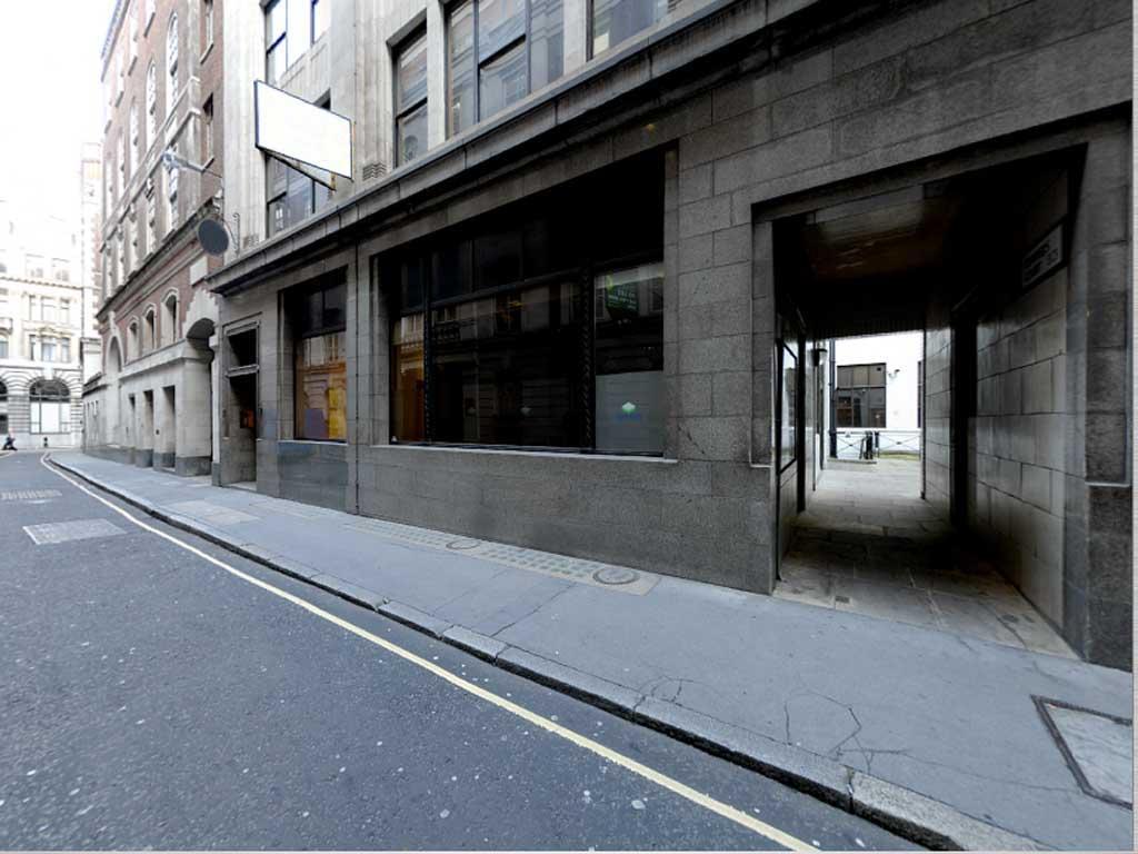
196

197

198

199

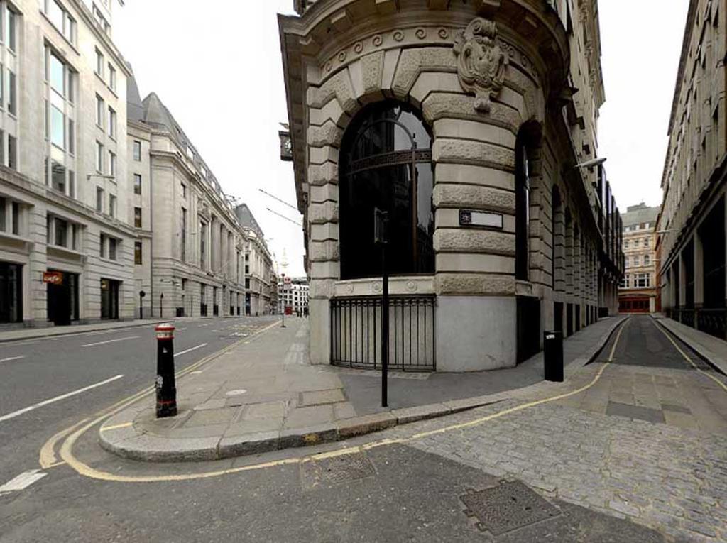
200

201

202

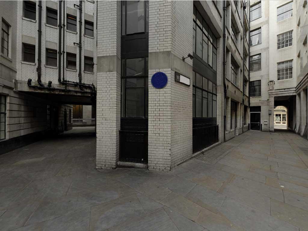
203

204

205

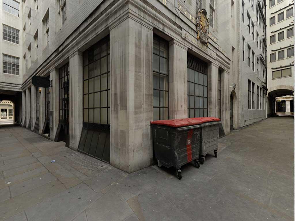
206

207

208 194

209 Appendix C Path connectivity in the stimulus set 195

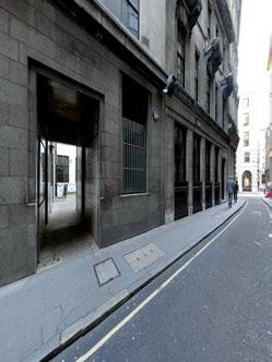
210 '3&4&!"#$%"&'()*+,%-#(&.#/%"&'()*+,%-#(& '3&5&!"#$%"&01#2/*&.#/%"&01#2/*&!"#$%"&'()*+,%-#(&.#/%"&'()*+,%-#(&!"#$%"&01#2/*&.#/%"&01#2/*&!"#$%"&'()*+,%-#(&.#/%"&'()*+,%-#(&!"#$%"&01#2/*&.#/%"&01#2/*& '3&6&!"#$%"&'()*+,%-#(&.#/%"&'()*+,%-#(& '3&7&!"#$%"&01#2/*&.#/%"&01#2/*&!"#$%"&'()*+,%-#(&.#/%"&'()*+,%-#(& '3&88&!"#$%"&01#2/*&.#/%"&01#2/*&!"#$%"&'()*+,%-#(&.#/%"&'()*+,%-#(&!"#$%"&01#2/*&.#/%"&01#2/*& '3&84&!"#$%"&'()*+,%-#(&.#/%"&'()*+,%-#(& '3&85&!"#$%"&01#2/*&.#/%"&01#2/*&!"#$%"&'()*+,%-#(&.#/%"&'()*+,%-#(& '3&86&!"#$%"&01#2/*&.#/%"&01#2/*&!"#$%"&'()*+,%-#(&.#/%"&'()*+,%-#(&!"#$%"&01#2/*&.#/%"&01#2/*&

211 '3&87&!"#$%"&'()*+,%-#(&.#/%"&'()*+,%-#(& '3&98&!"#$%"&01#2/*&.#/%"&01#2/*&!"#$%"&'()*+,%-#(&.#/%"&'()*+,%-#(& '3&94&!"#$%"&01#2/*&.#/%"&01#2/*&!"#$%"&'()*+,%-#(&.#/%"&'()*+,%-#(&!"#$%"&01#2/*&.#/%"&01#2/*& '3&95&!"#$%"&'()*+,%-#(&.#/%"&'()*+,%-#(& '3&96&!"#$%"&01#2/*&.#/%"&01#2/*&!"#$%"&'()*+,%-#(&.#/%"&'()*+,%-#(&!"#$%"&01#2/*&.#/%"&01#2/*&

212 198

213 Appendix D Questionnaires 199

214 Thank&you&for&agreeing&to&participate.&This&is&a&desktop5based&experiment&that& lasts&less&than&10&minutes;&it&is&divided&into&two&parts.&results&collected&will&be& anonymous&and&will&contribute&to&my&research.&& & Participant&Questionnaire& Gender&& & & M& F& Are&you&a&student&&& Y& N& If&yes,&what&is&your&field&..& & Participant&Instructions& When&you&are&ready&the&experiment&will&begin.&& You&will&be&presented&will&a&series&of&images&of&street&junctions.&Each&image&will& show&you&a&decision&point&with&a&clear&left/right&option.&you&will&be&asked&to& make&a&choice&to&go&either&left&or&right,&according&to&a&task&that&will&be&given&to& you&below.&you&should&respond&as&soon&as&you&have&made&your&choice,&by&hitting& the&arrow&keys&on&the&keyboard.& & Part&1.&When&looking&at&each&image&please&respond&to&the&following&task:& Which%way%would%you%go?% & & Part&2.&When&looking&at&each&image&please&respond&to&the&following&task:& You%are%looking%for%a%taxi%rank.%Which%way%would%you%go?% &

215 This study examines what we look at in cities. It is part of ongoing research between the architecture and science departments of UCL. By participating you are contributing to this research. In the study you will put on a piece of equipment that looks like a pair of glasses. It will track your eye movements and works best if you don t wear glasses when watching a screen. The study will take less than 10 min. If you would like to participate, please fill in the following questionnaire. All data is collected solely for the purposes of the study. Gender M F Participant Questionnaire Age.. Do you usually wear glasses to watch a screen (eg. TV?) Yes No Race: (eg. White European, British Indian, Afro-Caribbean etc.) Profession.. Annual Salary (0-20k; 20-40k; 40-60k; 60+) In what country did you grow up? In what country do you live now?. If different, how old were you when you moved?.. Participant Instructions The equipment will be fitted onto you and needs to be carefully calibrated, to make sure it s working properly. When you are ready the experiment will begin. You will see a number of images of a city. Please look at each one carefully. At the end you will be asked a few general questions.

216 !"#$"% &'( ) *+," &'( )! "# $%& '()*+,-).//0-1 %!"#$"%/ 2 "" "3& ' :;<8).=.4> % 7<?*=-9 #3 %@@&!< 8).=.4><'().:-1 % ""< "#< 2< 8).=.4><A1B (/-0",-).//0-1 % 16-< 7@C33,>.1040 % D-=.1<'E0).:-1 % 2-9-F % ##1+2/3+2+%4 &'( ) 5%'6"778'# &'( ) G>.=0<HI)*J0-1 K5 3@ 35C$& '::*I1=-1= 7 #3 %@@& 5@<+<"@; %$ ')=.4= L "@<+<3@; # M*:=*) " 3@;N # H90:=).: !-:=*)F<O*);0) 5 #3 %@@& P*I40O.( Q-11F 5 QI)40 5 R=IB01= 5$ 53&?0-:>0) L R:>**9:>.9B %% S=>0) 53 5L& #3 %@@& 53< -##1+2/3+2+%4/ #< #< 5@<+<"@;< %%< %$< 3@< "@<+<3@;< 3@;N< 16-< L< *+,"/ %< 5<%<%<5<%<%<%<%< 7< K5< 5%'6"778'#/ 7< L< "< 5< 5< 7< 5$< 5< 5< 5< '()*+,-).//0-1< '4.-1< 89-:;<8).T4>< 8).T4><'().:-1< 8).T4><A1B.-1<,-).//0-1<,>.1040< D-T1<'E0).:-1< 2-9-F< '::*I1=-1=< ')T4=< M*:=*)< H90:=).:.-1<!-:=*)F<O*);0)< P*I40O.(0< 16-< Q-11F< QI)40< R=IB01=<

217 Appendix E Fixation data - spatial tasks 203

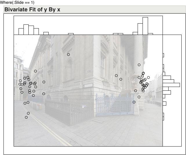
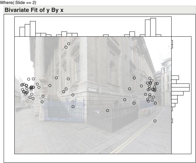
218

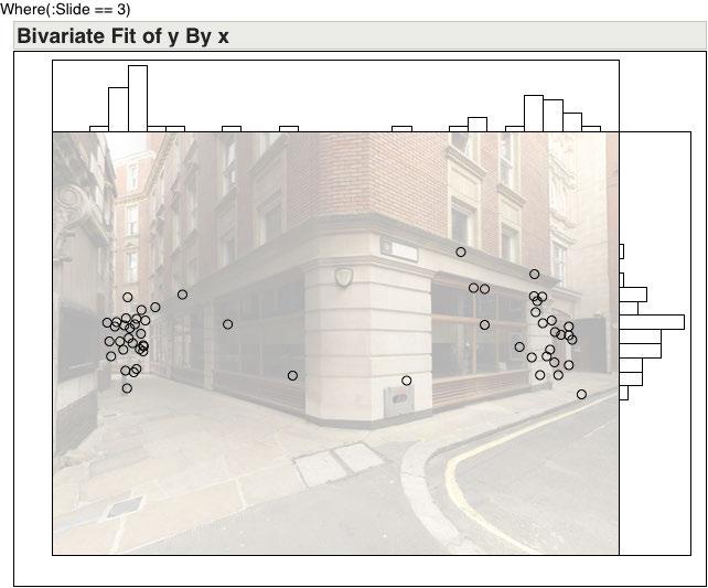
219

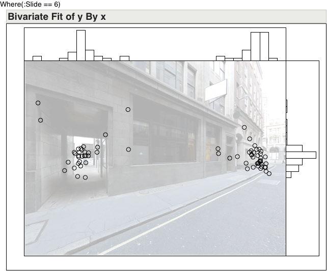
220

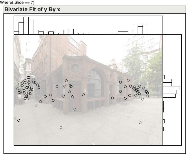
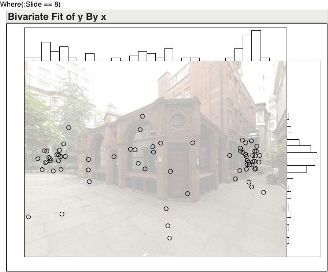
221

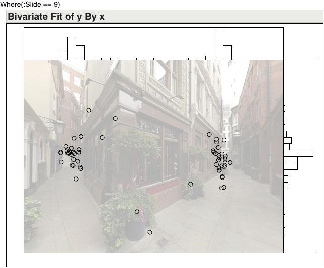
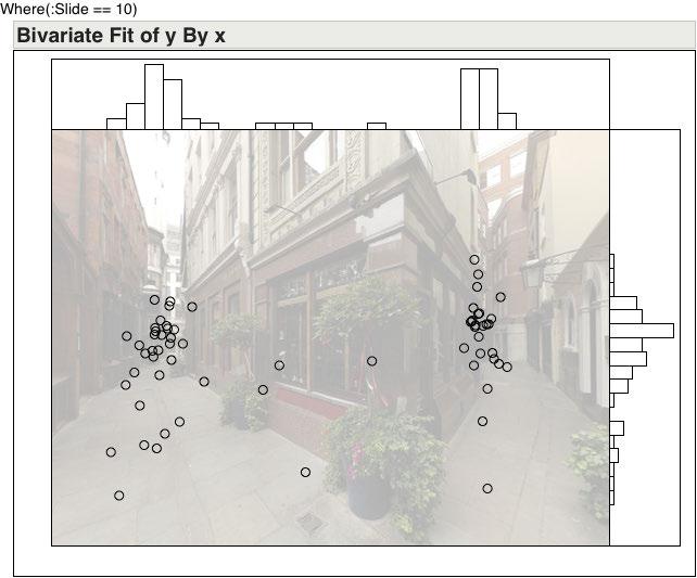
222

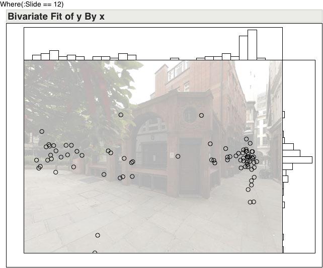
223

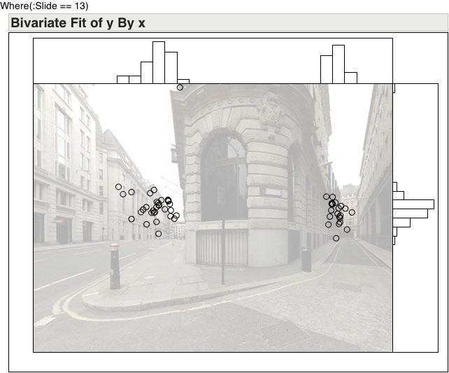
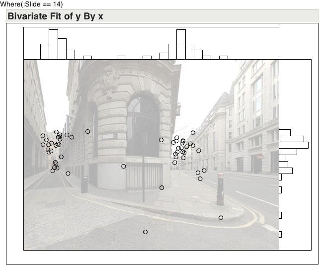
224

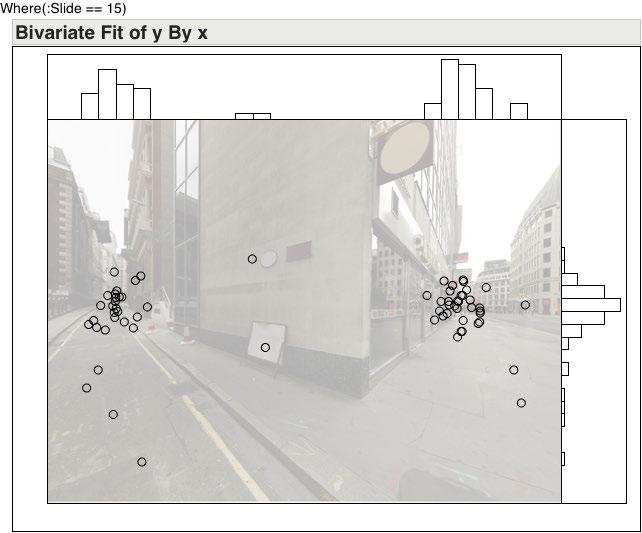
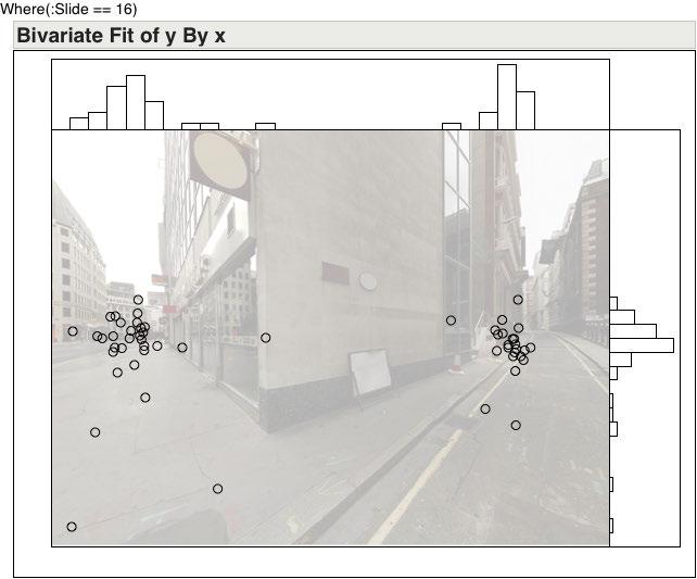
225

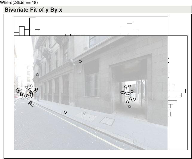
226

227

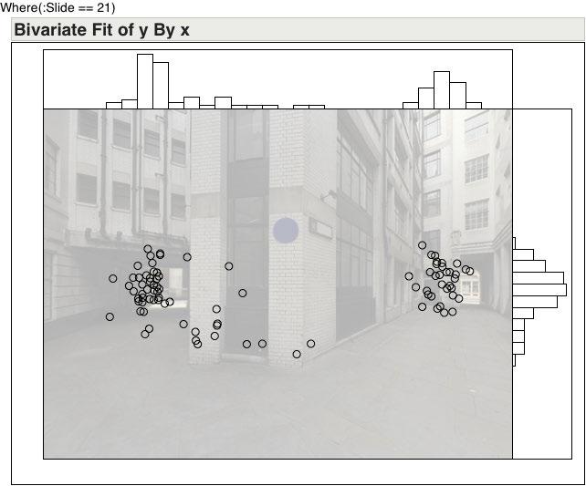
228

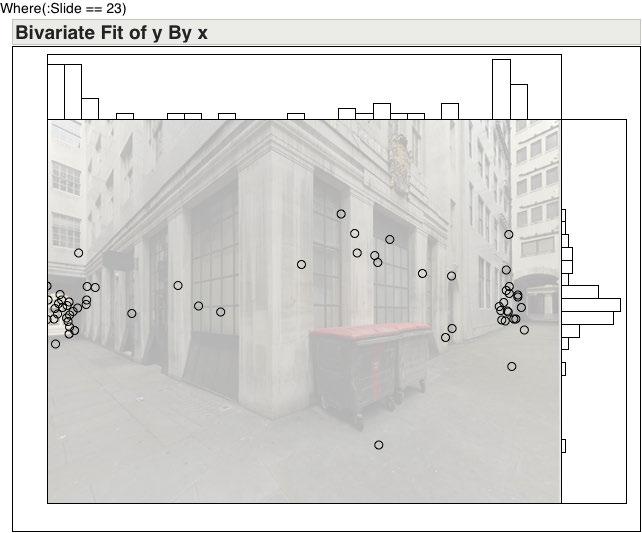
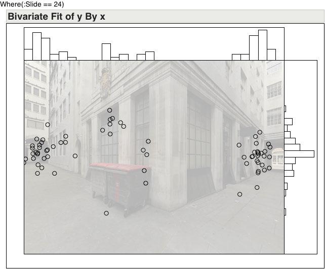
229

230

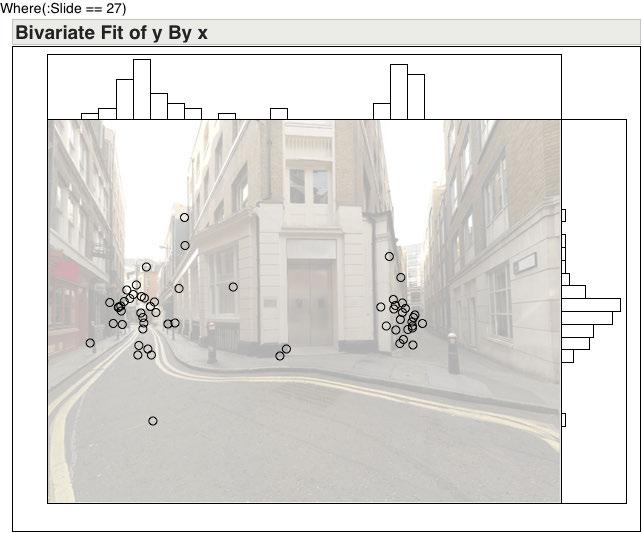
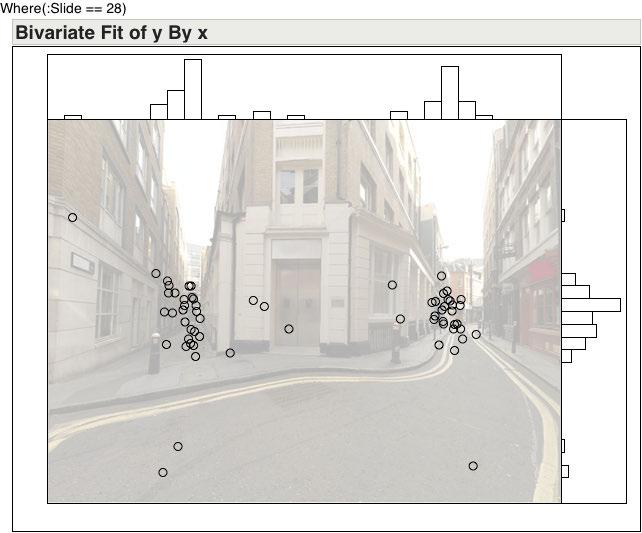
231