Improving Causal Claims in Observational Research: An Investigation of Propensity Score Methods in Applied Educational Research

Transcription

1 Loyola University Chicago Loyola ecommons Dissertations Theses and Dissertations 2016 Improving Causal Claims in Observational Research: An Investigation of Propensity Score Methods in Applied Educational Research Julie Diane Wren Loyola University Chicago, Recommended Citation Wren, Julie Diane, "Improving Causal Claims in Observational Research: An Investigation of Propensity Score Methods in Applied Educational Research" (2016). Dissertations This Dissertation is brought to you for free and open access by the Theses and Dissertations at Loyola ecommons. It has been accepted for inclusion in Dissertations by an authorized administrator of Loyola ecommons. For more information, please contact This work is licensed under a Creative Commons Attribution-Noncommercial-No Derivative Works 3.0 License. Copyright 2016 Julie Diane Wren

2 LOYOLA UNIVERSITY CHICAGO IMPROVING CAUSAL CLAIMS IN OBSERVATIONAL RESEARCH: AN INVESTIGATION OF PROPENSITY SCORE METHODS IN APPLIED EDUCATIONAL RESEARCH A DISSERTATION SUBMITTED TO THE FACULTY OF THE GRADUATE SCHOOL IN CANDIDACY FOR THE DEGREE OF DOCTOR OF PHILOSOPHY RESEARCH METHODOLOGY BY JULIE D. WREN CHICAGO, ILLINOIS MAY 2017

3 Copyright by Julie D. Wren, 2017 All rights reserved.

4 ACKNOWLEDGMENTS I would never have been able to finish my dissertation without the guidance of my committee members, the support of my family and the love of my son. I would like to express my deepest gratitude to my advisor, Dr. Terri Pigott, her guidance and patience were essential for helping me move this work forward. Additionally, I would like to thank Dr. Susan Farrugia and Dr. Meng-Jia Wu for their feedback throughout this process. Special thanks to the institution that was willing to share their student data to complete this work. None of this would be possible without the support of my family particularly the village of women that helped to raise my son while I was at class or working on my dissertation, Thank you to two amazing grandmothers, Eizabeth and Kathy, along with an entourage of aunts, Natalie, Kelly, Katie and Kristin. Finally, thank you to my son who gleefully went from daycare to family so his mom could work and continue her studies. iii

5 For my son, Kelan.

6 It takes a village.

7 TABLE OF CONTENTS ACKNOWLEDGMENTS TABLE OF CONTENTS LIST OF FIGURES LIST OF TABLES LIST OF TERMS iii vi vi vii viii CHAPTER ONE 1 Observational Research 2 Statement of the Problem 3 Causal Claims in Observational Research 3 Propensity Score 4 Purpose of the Study 6 Research Questions 7 Delimitations. 8 Limitations. 8 Significance of the Study 8 Anticipated Outcomes 10 CHAPTER TWO 11 Rubin s Causal Model (RCM) 11 Assumptions 13 Stable Unit Treatment Value Assumption. 13 Strongly Ignorable Treatment Assignment. 14 Criticisms 14 Design Choice and Causal Inference 15 Randomized Experiments 15 Observational (nonrandomized) Research 16 Causal Local institution in Observational Research 17 Alternative Designs 18 Applied Statistical Analysis 19 Controlling for Covariates. 20 Creating Equivalent Groups. 21 The Propensity Score 22 Covariate Selection 22 Estimating the Propensity Score 23 Conditioning the Propensity Score 24 Matching. 25 Stratification. 27 vi

8 Weighting 27 Covariance adjustment 28 Assessing the Treatment Effect 28 Evaluating Accuracy of the Propensity Score 28 Considerations for the Application of Propensity Score 29 Covariate Concerns 29 Estimation Methods 30 Accuracy of Propensity Score Methods 31 Effectiveness of the Propensity Score Model 32 PSM in Higher Education 33 Multi-institutional Research 34 Single Institution Research 35 Overall Aim of Research 37 CHAPTER THREE 39 Study Overview 39 Research Questions 40 Design 41 Data Collection 42 Student Information System (SIS). 42 Entering Student Survey Dataset 43 Noncognitive Survey Dataset 43 Research Population 43 Variables 44 Analytic Procedures 45 Step one: Determine the difference between groups 45 Step two: Estimate the propensity score 45 Step three: Assess the region of common support 46 Step four: Propensity Score Conditioning 47 Step five: Assessment of balance 47 Step six: Estimate the ATE 48 Step seven: Sensitivity analysis of unobserved covariates 48 Comparison across models 49 Chapter Summary 49 CHAPTER FOUR 50 Step zero: Baseline data 50 Step one: Determine the difference between groups on the selection variable 51 Step two: Estimate the propensity score 57 SIS Model 57 SIS+ESS Model 59 SIS+NCS Model 64 SIS+ESS+NCS 67 Summary 73 Step three: Assess the region of common support 74 vii

9 SIS Model 74 SIS+ESS Model 76 SIS+NCS Model 77 SIS+ESS+NCS Model 79 Summary 80 Step four: Propensity Score Conditioning 80 Step five: Assessment of balance 82 Step six: Estimate the ATE 84 Step seven: Sensitivity analysis of unobserved covariates 85 Chapter Summary 92 CHAPTER FIVE 93 Summary of the Study Purpose 93 Research Questions 93 Method 94 Discussion of the Study s Results 95 Group Differences Prior to Estimation 95 Estimation of the Propensity Score 96 Conditioning strategies 97 Covariate Balance 99 Treatment Effect 100 Limitations 101 Practical Implications 102 Covariate Selection Matters 102 Conditioning Strategy Matters 103 Balance Assessment Strategy Matters 104 Sensitivity of the ATE Matters 104 Future Research 105 APPENDIX A 107 APPENDIX B 112 APPENDIX C 115 APPENDIX D 125 REFERENCE LIST 175 viii

10 LIST OF FIGURES Figure 1. Region of Common Support: SIS Model 75 Figure 2. Region of Common Support - Box Plot: SIS Model 75 Figure 3. Region of Common Support: SIS+ESS Model 76 Figure 4. Region of Common Support - Box Plot: SIS+ESS Model 77 Figure 5. Region of Common Support: SIS+NCS Model 78 Figure 6. Region of Common Support - Box Plot: SIS+NCS Model 78 Figure 7. Region of Common Support: SIS+ESS+NCS Model 79 Figure 8. Region of Common Support - Box Plot: SIS+ESS+NCS Model 80 vi

11 LIST OF TABLES Table 1. Dropped variables across datasets 53 Table 2. Parameter Estimates for Logistic Regression 55 Table 3. Parameter Estimates for SIS Model 58 Table 4. Parameter Estimates for SIS+ESS Model 60 Table 5. Parameter Estimates for SIS+NCS Model 65 Table 6. Parameter Estimates for SIS+ESS+NCS Model 68 Table 7. Summary of PS Models 74 Table 8. Description of Matching Schemes and Resample Size 81 Table 9. Covariate Balance across Matching Schemes 82 Table 10. Average Treatment Effect across Matching Schemes. 84 Table 11. Sensitivity Analysis 86 Table 12. Sensitivity Analysis, Unobserved Covariates: SIS Model 88 Table 13. Sensitivity Analysis, Unobserved Covariates: SIS+ESS Model Error! Bookmark not defined. Table 14. Sensitivity Analysis, Unobserved Covariates, SIS+NCS Model 90 Table 15. Sensitivity Analysis, Unobserved Covariates: SIS+ESS+NCS Model 91 Table 16. Significant Covariates across PS Models 96 Table 17. Percentage of Pairs Lost from Same PS Model, No Caliper 98 vii

12 LIST OF TERMS The following definitions are quoted from the Integrated Postsecondary Education Data System (IPEDS) glossary and are available at slight modifications were made to fit the current format. Cohort refers to a specific group of students established for tracking purposes. Credit hour refers to a unit of measure representing the equivalent of an hour (50 minutes) of instruction per week over the entire term. It is applied toward the total number of credit hours needed for completing the requirements of a degree, diploma, certificate or other formal award. Degree/certificate-seeking students refers to students enrolled in courses for credit who are recognized by the institution as seeking a degree or other formal award. Entering students (undergraduates) refers to students at the undergraduate level, both fulltime and part-time, coming into the institution for the first time in the fall term (or the prior summer term who returned again in the fall). This includes all first-time undergraduate students, students transferring into the institution at the undergraduate level for the first time, and non-degree/certificate seeking undergraduates entering in the fall. First-time students (undergraduates) refers to students who have no prior postsecondary experience (except as noted below) attending any institution for the first time at the undergraduate level. This includes students enrolled in academic or occupational programs. It also includes students enrolled in the fall term who attended college for the first time in the viii

13 prior summer term, and students who entered with advanced standing (college credits earned before high school graduation). Four-year institutions refers to postsecondary institutions that offer programs of at least four years duration or programs at or above the baccalaureate level. Thus, schools that offer post baccalaureate certificates only or those that offer graduate programs only are also included. In addition, free-standing medical, law or other first-professional schools are considered four-year institutions. Fall cohort refers to the group of students entering in the fall term established for tracking purposes. Fall term refers to the part of the academic year that begins between late August and November 1. Fulltime students (undergraduates) refers to students enrolled for 12 or more semester credits, or 12 or more quarter credits, or 24 or more contact hours a week each term. Postsecondary education refers to the provision of a formal instructional program whose curriculum is designed primarily for students who are beyond the compulsory age for high school. This includes programs whose purpose is academic, vocational, and continuing professional education, and excludes vocational and adult basic education programs. Public institutions refers to educational institutions whose programs and activities are operated by a publicly elected or appointed school official and are primarily supported by public funds. Undergraduate refers to a student enrolled in 4- or 5-year bachelor s degree program, an associate degree program or a vocational or technical program below the baccalaureate. vi

14 CHAPTER ONE INTRODUCTION Educational researchers often face the challenge of determining the efficacy of a program, treatment, or intervention (hereto referred to as treatment) on a desired outcome (Murnane & Willett, 2011). These research questions often aim to explain whether or not treatment X caused outcome Y, but to investigate causal relationships, three requirements must be met. The requirements are: (1) the cause must precede the effect, (2) the cause must be related to the effect, and (3) no other plausible explanation exists except the causal explanation (Shadish, Campbell, & Cook, 2002, p.6). Although the first two requirements are relatively straightforward, the third requirement is much more difficult to ascertain. The need to rule out all other probable explanations to make a causal claim is why random assignment is referred to as the gold standard (Murnane & Willett, 2011; Shadish, Campbell & Cook, 2002). Random assignment, if employed properly, has the benefit of balancing the observed and unobserved covariates between groups, making any differences between the groups arbitrary (Rubin, 1974, p. 694). This balancing ability of random assignment is critical as it ensures that the groups are equal in expectation thus bolstering confidence that the third requirement of causation, no other plausible explanation exists except the causal explanation, has been met. Although random assignment provides the best support for ensuring that there are no other probable explanations, randomized experiments are less common in educational research due to 1

15 financial, practical and ethical concerns (Murnane & Willett, 2011; Shadish, Campbell & 2 Cook, 2002). These challenges and concerns have led to a reliance on observational research for educational inquiry. Observational Research Since observational research does not involve random assignment, it is subject to selection bias (Shadish, Campbell & Cook, 2002). Selection bias is systematic bias that results from individuals electing rather than being assigned to participate. Consider a new curriculum developed to improve reading levels. In the school where the reading program was administered, students whose parents signed them up to participate received the curriculum. At the end of the year, the students that participated in the program had demonstrated higher reading scores. Although the reading program might have had to led to these improvements, it is possible that other factors led to these differences. Taking a look at the two groups of students, students who participated in the reading program were more likely to be female and have more than 50 books in the home and less likely to demonstrate financial need. Rather than the differences in the treatment outcome resulting from the reading program, the improvements might be the result of the financial, social and educational advantages the children who participated were afforded by birth rather than the program. In this instance, parental affluence would be a confounding variable. To determine the impact of the program on performance, the variation in the outcome due to the confounding variable must be controlled for or removed from the analysis. Observational research does not, by design, provide substantial evidence that there are no other probable explanations. Therefore, there is incongruence between the most popular design

16 choice and the needs of educational researchers. Educational researchers need to be able to 3 attest to the impact of treatment on individuals; therefore, the study of methodological and/or statistical approaches to allow for the investigation of causal inference is both critical and necessary. Statement of the Problem Due to the expense and ethical concerns associated with randomized research, causal questions are often addressed without the benefits of random assignment. Often, researchers attempt to minimize the impact of selection bias by controlling for the differences between groups on key covariates with regression (Morgan & Winship, 2007). Unlike random assignment, where the balancing between groups occurs before the analysis, regression balances and analyzes at the same time. While regression can provide information about the association between a treatment and an outcome, it cannot substantiate causal claims when used alone. Causal Claims in Observational Research Although regression, used as a statistical tool, does not allow for causal claims, it is powerful when combined with alternative design features such as regression discontinuity and instrument variable estimation. Regression discontinuity exploits exogenous characteristics of a treatment to support causal claims (Thistlethwaite & Campbell, 1960). Again, consider the new reading program. If a cutoff score was required for participation, then regression discontinuity could be employed. The cutoff score serves as the exogenous characteristic, and the analysis would focus on the students at and around the cutoff. The exogenous characteristic is both a necessary and limiting aspect of regression discontinuity. It is necessary because focusing on this smaller area, just around the cut off, allows for causal claims to be made.

17 Although causal claims can be made, they are bounded to the individuals closely surrounding 4 the cutoff score, limiting generalizability and resulting in a local average treatment effect (Thistlethwaite & Campbell, 1960). Propensity Score In addition to alternative design features, statistical procedures that do not require design modifications can be employed. Based on the early work of Neyman in 1923 and Fisher in 1925, Rubin (1974) developed Rubin s Causal Model (RCM). Rubin framed all investigations of causal relationships as a missing data issue. Consider the new reading program; regardless of whether students are randomly assigned, students are signed up by their parents, or a cut off score is employed, each student can only be observed in one condition. Therefore, a student that is participating in the new reading program cannot also be observed for not participating in the new reading program. So for each student that participates in the reading program the outcome is known; but for that same student, the outcome for not participating in the reading program is unknown. This is why causal inference can be conceptualized as a missing data problem. Since the missing data can never be fully known, the goal becomes devising a set of conditions in which the missing data can be closely approximated. Although random assignment is the gold standard, it is not always feasible or desirable. When random assignment is not possible, the principles, derived by Rubin (1974), can be applied to model the bias (i.e., selection process) (Rosenbaum & Rubin, 1983a). Modeling the selection process has the advantage of approximating random assignment because, like random assignment, the selection process is analyzed prior to the outcome. Consider the new reading

18 program; parents had chosen whether or not to have their children participate, and initial 5 results indicated a favorable outcome among students in the reading program. Although there was a positive treatment effect, it is unclear whether or not the outcome is a result of the reading program or the selection process because there were significant differences between the groups at the outset of the study. Rather than controlling for these observed differences between groups, which is a common strategy, the selection process can be modeled. Regression is often used to model the selection bias with the summation of this process resulting in a single score, known as a propensity score. A propensity score is the conditional probability of assignment to a particular group, given a vector of covariates (Rosenbaum & Rubin, 1983 p. 42). Propensity score methods are different than regression because they use a single value to create non-equivalent groups. Therefore, unlike regression, the bias between the groups before and after propensity score methods can be assessed. Although propensity score methods offer an alternative to experimental designs for causal analysis, its utility is based upon successfully proving that the two assumptions have been met: the stable unit treatment value assumption (SUTVA) and strongly ignorable treatment assignment (Rosenbaum & Rubin, 1983a; Rubin, 1980). The SUTVA assumption asserts that there is only one version of treatment and no interference between units (Cox, 1958, p. 19; Rubin, 1980, p.591). This means that the outcome of one unit is not impacted by the treatment of another unit, leaving only two potential outcomes (Little & Rubin, 2000, p.123). In addition to SUTVA, there has to be a strongly ignorable treatment assignment, also known as independence (Rosenbaum & Rubin, 1983a). The assumption of independence requires that

19 the determination of cause (treatment or control) to which a unit is exposed is unrelated to all 6 other variables (Holland, 1986, p.458). Stated alternatively, the treatment assignment is exogenous. Since there is no direct statistical test to ensure that these assumptions have been met, the quality of the methodology and related statistical analysis help to build support that these assumptions have been met. Purpose of the Study Although propensity score methods are conceptually simple and easy to understand, ensuring that the selection process is strongly ignorable is a challenge. This study used existing institutional data from a large, urban, public, very high research university to compare sixteen matching schemes, built from three separate datasets, to estimate the propensity score, achieve balance between groups and test the sensitivity of the average treatment effect (ATE). For each PS model, four different conditioning strategies were applied. The first four matching schemes used commonly collected data available within a student information system (referred to as SIS dataset). The next four matching schemes combined the SIS dataset with data from an entering student survey (referred to as ESS dataset). The next four matching schemes, again, combined the SIS dataset with data gathered from a noncognitive survey (referred to as NCS dataset). The final four matching schemes included data from the SIS, ESS and the NCS datasets. Each model builds upon the next, offering additional covariates for the model building process. To assess the effectiveness of these propensity score techniques in an applied educational research setting, the methodological research questions are nested within the framework of an overarching contextual research question. This guiding research question aimed to understand

20 7 the extent to which first-time, fulltime students who enrolled in optimal credit levels (defined as 15 or more credit hours during the first term of attendance) experienced greater levels of success. Student success is a complex phenomenon and includes multiple and sometimes competing constructs. This research uses first-year retention as a proxy for student success. Students are considered retained if they were enrolled at the university, the following fall term. Many researchers have studied retention resulting in various models with a diverse set of covariates (e.g., Pascarella & Terenzini, 2005; Ting, 1998; Tinto, 1975; 1993). Although this research does not seek to understand the complexity of student success, it does try to understand the influence the availability of additional covariates has on propensity score techniques and their influence on the stability of findings in applied educational research. Research Questions 1. To what extent do the treatment and the control groups vary naively across covariates? 2. To what extent do different PS models achieve overlap between the treatment and control groups? 3. To what extent do different PS models and conditioning strategies impact the sample size? 4. To what extent do different PS models and conditioning strategies achieve balance between groups? 5. To what extent do different PS models and conditioning strategies reach the same overall conclusions? 6. To what extent is the average treatment effect robust against unobserved covariates under different PS models and conditioning strategies?

21 Delimitations. Delimitations of the study include: 8 1. The study was limited to a large, public, very high research postsecondary institution; therefore, results are not generalizable to other postsecondary institutions. 2. The study was limited to first-time, fulltime students and does not offer information about transfer students or part-time students. 3. Conclusions drawn from the analysis were based solely on student factors that are measurable; other aspects of the student experience derived from a qualitative approach were not included. 4. Each of the conditioning strategies used nearest neighbor, greedy, matching. As a result, no information can be garnered about performance relative to other strategies. Limitations. Limitations of the study include: 1. Continuation of the analysis is dependent on the performance throughout. 2. Survey data are not an integrated part of the student record system. Therefore, data loss exists as a result of varied survey participation among students. 3. Survey data were gathered using self-report measures. These data only represent students self-perceptions, and these perceptions are not corroborated by any behavioral indices or additional reporters. Significance of the Study This study adds to a growing body of knowledge of the significance of expansive covariate sets and the impact of propensity score techniques in applied educational research. Additionally, it contributes to an underdeveloped area of research, the use of propensity score methods in applied postsecondary institutions. Previous research has demonstrated that simply

22 controlling for covariates does not replicate findings from randomized experiments (Angrist & 9 Pischke, 2009). Therefore, there is a need to explore alternative methodologies for answering routine causal questions that arise in educational research. Despite the rapid growth of propensity score methods in education, there have been relatively few studies focused on issues within higher education. Those studies that have occurred typically adopt a single-level model (e.g., Clark & Cundiff, 2011; Dehejia & Wahba, 1999) use logistic regression for estimation (e.g., Clark & Cundiff, 2011; Schafer, Wilkinson & Ferraro, 2013; Vaughan, Lalonde & Jenkins-Guarnierie, 2014), and condition the propensity score using matching or stratification (e.g., Clark & Cundiff, 2011; Schafer, Wilkinson & Ferraro, 2013; Vaughan, Lalonde & Jenkins-Guarnierie, 2014). Although there has been some attempt to broaden the application of propensity score methods to hierarchical relationships in this context, studies using multilevel modeling are far fewer (e.g., Vaughan, Lalonde & Jenkins-Guarnierie, 2014; Heil, Reisel & Attewell, 2014). Further, most of the research in this area has focused on a specific research question rather than on the method itself. Although information about the use and utility of propensity score methods exists, based on research using simulated data or multiple arms studies with randomized research as one of those arms, there lacks knowledge about what works within the context. Additionally, there is limited information about how the availability of expansive variable sets can influence the conclusions of a study. Additionally, not much research has been done on the use of propensity score methods within a single institution, which is of interest to practitioners. When a single institution has been the focus of a research study, many of the necessary elements to judge quality are not

23 included (Ali et al., 2015; Thoemmes & Kim, 2011). This research adds to information about 10 the potential value of expansive datasets while detailing each of the steps for performing and assessing propensity score techniques. Anticipated Outcomes Although this study was explorative in nature, differences between the matching schemes were expected. Based on previous research (Steiner, Cook, Shadish and Clark, 2010; Steiner & Cook, 2013), the addition of relevant covariates was expected to impact the findings at various stages of analysis. The inclusion of additional covariates was expected to lead to stronger PS models that better accounted for the selection bias ultimately bolstering confidence in the study s conclusion. Despite this, the inclusion of the additional covariates was expected to negatively impact sample size and match rate. Although sample loss was expected as more restrictions were placed on the conditioning strategy (i.e., caliper widths), it was unclear whether the conditioning strategies would perform differently across PS models.

24 CHAPTER TWO REVIEW OF LITERATURE This study investigated the availability of an expansive covariate set on propensity score (PS) models and the behavior and performance of propensity score conditioning strategies in applied educational research. Accordingly, the review focuses on causal local institution and the use of propensity score methods in observational research and their appropriateness and utility in applied educational research. To provide a foundation, the historical roots of causal inference and its extension to observational research through Rubin s Causal Model (RCM) are explained. Next, research design choices that aim to understand causal relationships are explored followed by a discussion about the logic and use of the propensity. Additionally, a synthesis of current recommendations for applying propensity score methods and the use of propensity score methods in higher education are discussed. Lastly, the empirical gaps are identified and the ability of this research to bridge this gap will be addressed. Rubin s Causal Model (RCM) With roots predating the 16 th century, modern science and experimentation evolved from philosophy taking foothold in the 17 th century (Shadish, Cook, & Campbell, 2002). As interest moved away from observations about the world, interest moved toward active manipulations and their effect on the phenomenon understudy. As knowledge and interest in experimntation grew so did the desire to control extraneous variables and minimize bias. By the early 1900s, this coalesced into the development of the modern experiment, including both random assignment 11

25 12 and control groups (Shadish, Campbell & Cook, 2002). This desire to maximize control helped to make causal inference synonymous with randomized experiments, and it was not until 1974 that causal reasoning was first applied to observational research (Rubin, 1974). Rubin s Casual Model (RCM; Rubin 1974, 1978), with its potential outcome notation, is an extension of the work of both Neyman in 1923 and Fisher in 1925 (Rubin, 1990). RCM is also referred to as the potential outcomes framework and the counterfactual model of causal inference. Due to Rubin s significant application of this framework to observational research, it will be referred to as RCM throughout (Holland, 1986, p.946). Neyman developed a nonparametric model where each unit had two potential outcomes, and the difference between these outcomes was the causal effect. The specification of two outcomes is particularly helpful since the requirement of two causes (treatment, control) is often taken for granted (Holland, 1986, p.459; Yuke, 1903, p.126). The work of both Neyman and Fisher was rooted in experimental design and was first applied to nonrandomized research by Rubin (1974). RCM draws attention to the missing data issue formalized in the potential outcomes framework. More formally stated, let Y = the potential outcomes, Z= the indicator for treatment received, i = the unit, and j = the exposed treatment. Therefore, when (Z = 0, Y i 0 ) is the potential treatment outcome for the ith unit that received (Z = 0) treatment and (Z = 1, Y i 1 ) is the potential treatment outcome for the ith unit that received (Z = 1) treatment. Since a unit cannot be observed in both conditions, Y i 1 and Y i 0 are referred to as potential outcomes. The goal of analysis is to compare these two potential outcomes (Y i 1, Y i 0 ) using an average treatment effect (τ). Depending on the nature of the investigation, the average treatment effect for the overall population (ATE), the average treatment effect for the treated (ATT) or the

26 13 average treatment effect for the untreated (ATU) might be of interest. The average treatment effect is defined as the expected difference in the potential outcomes with the following, ATE τ = E(Y 1 i Y 0 i ) = E(Y 1 i ) E(Y 0 i ) ATT τ T = E(Y 1 i Y 0 i Z i = 1) = E(Y 1 i Z i = 1) E(Y 0 i Z i = 1) ATU τ U = E(Y 1 i Y 0 i Z i = 0) = E(Y 1 i Z i = 0) E(Y 0 i Z i = 0) If both potential outcomes could be observed, then calculating the average treatment effect would simply be an average of the individual treatment differences. Since this is not the reality, the most that can be calculated is the treatment outcomes for the treated and the control outcomes for the untreated. The simple difference between these two outcomes provides a biased estimator of the average treatment effect. There is no statistical procedure or methodology that can fully resolve this missing data problem. Assumptions Since there is no way to completely resolve the missing data issue, there has to be a set of assumptions to allow for causal local institution. As Holland (1986) pointed out, a statistical solution is required in addition to the scientific framework. Specifically, the statistical solution needs to address how information from different units can be used to understand the impact of treatment by supplementing an average causal effect (p.457). The two assumptions necessary within the potential outcomes framework are: the stable unit treatment value assumption (SUTVA) and the strongly ignorable treatment assignment. Stable Unit Treatment Value Assumption. The SUTVA asserts that there is only one version of treatment and no interference between units (Cox, 1958, p. 19; Rubin, 1980, p.591). This means that the outcome of one unit is not impacted by the treatment of another unit, leaving

27 14 only two potential outcomes (Little & Rubin, 2000, p.123). This is an essential assumption to ensure that the treatment, as designed, is responsible for the causal effect. In practice, this can be violated. For instance, consider a summer treatment program for children with behavioral disorders where children are blind to their medication treatment, receiving either a placebo or active pill daily. It is possible that child A receiving a placebo pill could cause increased negative behaviors for child B because child A is disturbing child B due to child A s treatment assignment (placebo). This violation of SUTVA increases the potential outcomes for child B because child B s outcomes would be a function of whether child A received a placebo pill or not as well as his own treatment assignment. The number of outcomes increases exponentially with the number of units (Little & Rubin, 2000, p.123). Therefore, a strong claim for meeting SUTVA is required. Strongly Ignorable Treatment Assignment. In addition to SUTVA, there must be a strongly ignorable treatment assignment, also known as independence (Rosenbaum & Rubin, 1983a). Since units cannot be observed under both conditions, their assignment to treatment Z must be independent of outcomes (Little & Rubin, 2000, p.125). The assumption of independence requires that the determination of cause (treatment or control) to which a unit is exposed is unrelated to all other variables (Holland, 1986, p.458). Stated alternatively, the treatment assignment is exogenous. When treatment assignment is non-ignorable or endogenous, the selection mechanism must be incorporated into the analysis (Little and Rubin, 2000, p.127). The assignment of units to treatment must be known. Criticisms

28 15 Not all researchers support the use of RCM for making causal claims. One of the major opponents of the potential outcome framework adopted by Rubin is Pearl (2010). Pearl stated the following, one cannot substantiate causal claims from associations alone, even at the population level behind every causal conclusion there must lie some causal assumption that is not testable in observational studies (p. 99). Pearl (2009, 2010) advocates for a structural equation model basis of causality and has criticized RCM for its adoption of counterfactual reasoning. Despite these criticisms, Little and Rubin defend counterfactual reasoning and believe the quality of the assumptions, not their existence, is the issue (2000, p.123). Essentially, they advocate for the acceptance of causal claims when the conditions to which they are arrived at are strong, strengthening their validity. Design Choice and Causal Inference While both SUVTA and the ignorable treatment assignment assumptions must be met, how these assumptions are met is not prescriptive. Therefore, causal claims are possible with varied design choices because it is not the nature of causation that changes but, rather, the amount of control over the phenomenon understudy (Holland, 1986, p. 954). While causal local institution are possible under varied design choices, the clearest and simplest pathway is randomization (Fisher, 1925; Holland, 1986, p.946, Little & Rubin, 2000, p.127). Randomized Experiments Randomized experiments involve the assignment of units to treatment by a process known as random assignment (Shadish, Campbell, & Cook, 2002, p.12). It is this assignment strategy that makes the design so powerful; random assignment offers the strongest support for the assumption of ignorable treatment assignment because it ensures that the potential outcomes

29 16 (Y 0, Y 1 ) are independent of treatment assignment Z, that is (Y 0, Y 1 ) Z. Random assignment, if employed properly, has the benefit of balancing the observed and unobserved covariates between groups, making any differences arbitrary (Rubin, 1974, p. 694). Achieving balance means that the groups are equivalent in expectation. Therefore, the groups (treatment and control) are balanced across both observed and unobserved covariates. As early as 19711, when the President s Commission on Federal Statistics called for increased utilization of randomization in research, there was a premium placed on randomized experiments despite their practical difficulties, and they remain the gold standard (Cochran & Rubin, 1973, p. 417; Guo & Fraser, 2015). Although randomization provides strong evidence to make causal claims, it too can be flawed. Even if perfectly designed and executed, randomized experiments can result in biased estimates of the treatment effect due to drop out and failure to comply with treatment guidelines. Further, randomization is not always possible due to ethical, financial or other practical concerns (Murnane & Willett, 2011; Shadish, Campbell & Cook, 2002). So despite some of the advantages of the design, researchers might choose not to use a randomized study design and opt for a nonrandomized study design also known as observational research. Observational (nonrandomized) Research The absence of randomization places a study into the categorization of observational research (Shadish, Campbell & Cook, 2002). Although randomization does not occur, the goal of the research often remains the same, to investigate causal relationships (Shadish, Campbell & Cook, 2002, p.14). Since observational research does not exert the same control as randomized research (e.g., random assignment), differences between groups exist prior to treatment. This

30 17 difference, known as selection bias, makes it difficult to make causal claims between groups because units choose their treatment condition (Rubin, 1974, p.698). Stated otherwise, the potential outcomes (Y 0, Y 1 ) are not independent of treatment selection. In practice, an observational study occurs when random assignment has not been used to assign units to active or control. Consider enrollment in private or public elementary schools. Families choose which type of educational setting to enroll their children. The decision to enroll a child into these differing educational systems can include a complex set of covariates including preference, proximity, finances and parental educational obtainment. This ability to choose the educational setting, public or private, is selection bias. Without random assignment, the best researchers can do is identify and track these variables that are different between the groups, referred to as confounding variables, and attempt to minimize or account for their impact (Cochran & Rubin, 1973, p.418). Comparing the two treatment groups without statistical adjustment leads to a biased estimate of the treatment effect. Therefore, to make a causal claim an unbiased effect of the treatment needs to be achieved and selection bias must be addressed. Causal Local institution in Observational Research Although treatment assignment is not independent in observational research, the selection process can be modeled and used to remove the bias resulting from self-selection into treatment or control groups (Murnane & Willett, 2011; Shadish, Campbell & Cook, 2002). The modeling of the selection process is best guided by direct study of the selection phenomenon and supported through a rich set of covariates, X = (X 1,, X p ) (Steiner, Cook, Shadish & Clark, 2010). When the selection process is adequately modeled, the potential outcomes are independent of treatment conditional on X, (Y 0, Y 1 ) Z X.

31 18 Accounting for the selection bias allows for the difference between groups to be an unbiased estimate of the treatment effect. Consequently, the average treatment effect is then the difference in conditional expectations of the treatment and control group s outcomes. That is, ATE τ = E{E(Y Z = 1, X)} E{E(Y Z = 0, X)} = E(Y 1 i ) E(Y 0 i ) ATT τ T = E{E(Y 1 Z = 1, X)} E{E(Y 0 Z = 1, X)} = E(Y 1 i Z i = 1) E(Y 0 i Z i = 1) ATU τ U = E{E(Y 1 Z = 0, X)} E{E(Y 0 Z = 0, X)} = E(Y 1 i Z i = 0) E(Y 0 i Z i = 0) In theory, once the selection bias has been accounted for and the treatment selection has been determined ignorable, the difference between treatment and control groups now represents an unbiased estimate of the treatment effect. This is a much more complex process as there are no statistical tests to determine if the selection bias has been sufficiently addressed (Guo & Fraser, 2015). In fact, research has demonstrated that misspecified models of the selection process can increase the bias (Leon & Hedeker, 2007). Therefore, modeling of the selection process warrants careful attention. While making causal claims with observational research is possible, not all researchers choose to go down this path; some elect to simply acknowledge the limitations of the research, explicitly stating that causal claims cannot be made. When researchers are interested in causal relationships, there are two main methods for its study: alternative design features and applied statistical analysis (Murnane & Willett, 2011, Shadish, Cook & Campbell, 2002). Alternative Designs The study of causal relationships can occur in observational research when alternative designs are used, specifically the regression-discontinuity approach and instrumental variables estimation. Regression discontinuity exploits the selection process to provide unbiased causal

32 19 estimates (Shadish, Campbell & Cook, 2002) while instrumental variables estimation exploits a covariate, referred to as the instrument, to provide an asymptotically unbiased estimate (Murnane & Willett, 2011). Both methods allow for causal inference in observational research. Consider a reading intervention that uses a cut off score to assign students to treatment or control. Since students are assigned to rather than selecting into groups, the assignment mechanism, the cut score, is fully known and a regression discontinuity approach can be used. A shift of the mean or slope of the line at the cut off score, the assignment mechanism, indicates that there is a treatment effect (Shadish, Campbell & Cook, 2002). Although this type of design does not provide information about the full sample of students, it does provide causal evidence for the impact of the treatment for students around the cut off score. Whether using regression discontinuity or instrument variables estimation, a limitation is that little is known about the full range of outcomes. With instrument variables estimation, knowledge is limited to that accounted for by the instrument, and with regression discontinuity, it is limited to those around the cut off score (Murnane & Willettt, 2011; Shadish, Campbell & Cook, 2002). Applied Statistical Analysis In absence of being able to use experimental or alternative designs, the next route to studying causal relationships is through applied statistical analysis. This method rests on the assumptions stipulated by Rubin (1974) in making causal claims in observational research: both SUTVA and strong ignorable treatment assignment must be achieved. Therefore, causal claims based on applied statistical analysis rely heavily on appropriate covariate selection. This process should be grounded in theory and strong knowledge of the selection process to ensure that the covariates adequately model the selection process (Murnane & Willettt, 2011; Steiner, Cook,

33 20 Shadish & Clark, 2010). Murnane and Willettt (2011) advise that methods are not magic and warn that the subsequent methods applied are only as good as the covariates used to model the selection process (p.288). Failure to adequately model the selection process ensures the failure of any subsequent method. Controlling for Covariates. One way to account for selection bias is to use statistical methods that control for covariates (e.g., regression, analysis of covariance). Regression is the most common statistical technique for controlling for covariates (Murnane & Willett, 2011). Multiple linear regression estimates treatment effects by regressing the outcome on the covariates. Relevant covariates and an indicator for treatment as well as any interactions between the treatment variable and each of the covariates are regressed on the outcome. While regression is frequently employed in the literature, it is insufficient for meeting the criteria for making causal claims. Although controlling for covariates can create balanced groups across an observed set of covariates, the groups remain unequal in expectation due to hidden bias. This hidden bias results from achieving balance across only observed covariates meaning that systematic difference between groups on unmeasured covariates might remain. Statistical methods that control for covariates are unlike experimental designs because the outcome and selection bias are addressed simultaneously. With randomized designs, equivalent groups are created by design at the outset of treatment. Therefore, the potential outcomes are independent of the selection modeling. Since this does not occur with post hoc adjustment, making causal local institution are not possible because the assumption of a strongly ignorable treatment assignment has not been met.

34 21 Creating Equivalent Groups. Another strategy for accounting for selection bias involves the use of statistical procedures to minimize its impact by creating equivalent groups prior to analysis. When this strategy is properly employed, the potential outcomes are independent of treatment conditional on a set of covariates (X, (Y 0, Y 1 ) Z X). There are different strategies for doing this including stratification and multivariate matching. One way to reduce selection bias is to stratify on one or many covariates. Stratification takes a covariate or set of covariates and subdivides the sample on them (Murnane & Willettt, 2011). These strata are then used for the analysis to help minimize bias. This strategy works well with one or two covariates but becomes impossible due to data sparseness and lack of common support with increasing numbers of covariates (Murnane & Willettt, 2011). Multivariate matching is most commonly used when examining the ATT (Guo & Fraser, 2015). In this case, multivariate matching attempts to resolve the missing data issue by matching each unit in the treatment group to at least one unit in the control group that is identical or near identical on observed covariates. If the ATE were of interest, a similar process would need to occur for matching each unit in the control group to at least one unit in the treatment group. Since finding an identical matched pair is difficult, matching involves a series of decisions related to distance, strategy and selected algorithm (Guo & Fraser, 2015). Both multivariate matching and stratification offer a way to create groups that are equivalent in expectation allowing for causal local institution, but the complexity of data makes the approach impossible to use. Even with as little as ten covariates the possible combinations exceed one million (Guo & Fraser, 2015). This obstacle is why propensity score techniques are desirable and why they continue to grow in popularity (Thoemmes & Kim, 2011).

35 22 The Propensity Score Propensity score (PS) techniques have an advantage over multivariate matching as the propensity score is a single, balancing score derived from all of the observed covariates X. The propensity score can be estimated using various statistical procedures that provide a probability, including regression, discriminant analysis and decision tree (Guo & Fraser, 2015). The propensity score is the probability of a unit receiving a treatment conditional on a set of covariates, e(x) = P(Z = X) (Rosenbaum & Rubin, 1983, p. 42). If the treatment assignment is strongly ignorable given the propensity score e(x), then the potential outcomes are independent of treatment assignment given the propensity score, (Y 0, Y 1 ) Z e(x). Additionally, the propensity score is a balancing score with the joint distribution being equivalent in both the treatment and control groups, P(X Z = 1) = P(X Z = 0). While balance is automatically achieved in randomized experiments, balance needs to be created in observation studies. For the propensity score to be balanced, a variety of statistical procedures can be applied including but not limited to matching and stratification (Guo & Fraser, 2015). Since there are many ways to arrive and use a propensity score, both the estimation process and the various methods are detailed. Covariate Selection Appropriate covariate selection is essential for ensuring that the treatment assignment is independent; ultimately, satisfying the assumption of an ignorable treatment selection. In theory, all variables related to the selection process and outcomes need to be included but, in practice, there is no statistical test to ensure that this has been accomplished (Luellen, Shadish, & Clark,

36 ). Therefore, it is the responsibility of the researcher to ensure that an adequate model of the selection process has been developed. The selection of covariates is best guided by empirical study of the selection process and theory as well as a comprehensive set of covariates (Luellen, Shadish & Clark, 2005; Murnane & Willettt, 2011). Rosenbaum (2002) advocates for the inclusion of important covariates even if they do not reach the level of statistical significance between groups. Therefore, if a covariate is related to the selection process and/or outcomes, it should be retained even if the p value falls below the specified threshold of statistical significance. Although there is no way to assure that hidden bias has been eliminated, sensitivity analyses can be done to bolster support. Estimating the Propensity Score Estimating the propensity score is most commonly completed using binomial regression models (Luellen, Shadish & Clark, 2005). Binomial regression models are used for discrete choice outcomes (i.e., treatment participation, yes or no) and model the probability that the binary response is a function of a set of predictors. Unlike, the traditional use of regression that models the outcome of interest, propensity score methods use regression to model the selection process. Although logistic regression is most often employed, it assumes linearity between the independent variables and the log odds. Due to this requirement, alternative approaches have been explored (Luellen, Shadish & Clark, 2005). To accommodate for the complex relationship between the selection process and covariates, statistical learning algorithms, such as random forest, regression trees or boosting, have been adopted (Westreich, Lessler & Funk, 2010). These statistical learning algorithms have advantages over traditional regression approaches because they are an automatic, nonparametric

37 24 procedure for addressing complex interactions and nonlinear relationships. Although they are better able to accommodate complex data, they have the tendency to lack fit when applied to new data (Luellen, Shadish & Clark, 2005). Regardless of the chosen estimation process, significant overlap between the propensity scores for the treatment and control group must exist. This area of overlap is referred to as the region of common support. When the distribution of the propensity scores is similar between groups, then all levels of the propensity score can be included (Guo & Fraser, 2015). When the distribution is dissimilar, propensity scores that fall outside the region of common support are dropped from subsequent analyses, a process often referred to as trimming. Sufficient overlap between the distribution of the propensity scores for the treatment and control groups must exist to continue with the analysis. If there is insufficient overlap, then the selection model might be misspecified and a re-estimation of the propensity score might yield different results. Overlap between the distributions of the propensity score must occur before moving to conditioning of the propensity score. Conditioning the Propensity Score Following the estimation of the propensity score, different conditioning methods can be applied. Conditioning methods aim to achieve balance between the treatment and control groups. There are different conditioning strategies that can be employed but these strategies influence the analysis of the outcome. For instance, matching (i.e., 1:1 and 1: many) and weighting by odds are commonly used when estimating the average treatment effect on the treated (ATT) (Austin, 2011). Full matching, stratification, inverse probability, propensity score weighting, ANCOVA and ANCOVA, including the propensity score as a covariate, are used when estimating the

38 25 average treatment effect (ATE) (Harder et al., 2010; Stuart, 2010; Steiner et al. 2010). Ultimately, the conditioning method chosen is important and it influences subsequent analyses. Matching. Matching is one method for conditioning the propensity score. Matching, in essence, is the pairing of similar units; units with a similar propensity score would be paired together. The unit in the control group would serve as the potential outcome had the unit in the treatment group not received the treatment. Most commonly, 1:1 matching is used. With one to one matching, a single treatment unit is paired with a single control unit. One-to-many matching is also employed; with this approach, a unit in the treatment group is matched to a specified number of control units. The equation below demonstrated a basic matching strategy: p i p j = min{ p i p k } Depending on the nature of the data, one matching strategy might be preferred to another. For instance, one-to-many is beneficial when there are a large number of control units, and the potential data loss is substantial. Consider the case where there were 100 units in the treatment group and 300 in the control. Despite the matching strategy, the maximum number of matches would be 100. With one-to-one matching, there would be substantial data loss since 200 control units would be dropped from the analysis. One-to-many matching has the ability to curtail this data loss by matching more control units to the treatment unit. While the matching strategy is an important consideration, the distance between matches is a critical consideration. Distance (δ) is a measurement of similarity between units on a given covariate, and this information is utilized within a matching strategy. The equation below shows a matching strategy that accounts for distance.

39 26 δ > 0 p i p j = min{ p i p k } Without setting this distance, also known as a caliper width, there is a potential for dissimilar units to be matched. Although caliper widths help to place some assurances around matching, it can cause a reduction in matching. In addition to these strategies, matching can also be done with or without replacement. Matching without replacement occurs, as discussed above, with one unit being matched to one treatment. When matching occurs without replacement, a control unit cannot be used again even if it matches well to more than one treatment unit. Therefore, matching with replacement can help increase balance between groups by allowing the same control unit to be matched to multiple treatment units. The downside to matching with replacement is that it again causes a loss in data. This loss in data is important because the conclusions might be less generalizable. Finally, the algorithm for matching needs to be determined. When matching with replacement, nearest matched to its nearest neighbor or set of nearest neighbors in the control group. When matching occurs without replacement, greedy or optimal matching can be used. Greedy matching is similar to nearest neighbor except once cases are matched; they are dropped from the dataset. Due to this first come strategy, some matches are not ideal because the overall distance is not minimized. To circumvent these issues, optimal matching can be used. Optimal matching ensures better overall matching by minimizing the global distance (Guo & Fraser, 2015). This means that some treated units are matched with their second, third or other best control units. Propensity score matching is similar to matching using multivariate methods, insomuch that propensity score matching can be done with variable distances using calipers, different

40 27 matching methods (e.g., 1:1 or 1: Many) and using various algorithms for nearest neighbor, optimal or greedy. The difference between the matching methods is that rather than using the entire set of covariates X, propensity score matching can use just the propensity score or the propensity and a subset of key covariates. Stratification. Alternatively, propensity score stratification can be employed which uses the estimated propensity score e (X) to divide the observations into distinct strata. Within each stratum, the units are homogenous; thus, the aim is to divide observations into groups with the same covariate distribution (Austin, 2011). Cochran (1968) demonstrated that 90% of overt bias is removed from a confounding variable when using 5 equal-size strata. This finding extends to the application of propensity score methods; Rosenbaum and Rubin (1984) additionally demonstrated that 90% of bias could be removed. Austin (2011) conceptualizes this strategy as 5 distinct quasi-randomized experiments. Treatment effects can be considered within a stratum or across strata. Typically, stratum-specific estimates of treatment effects are poled across stratum to estimate an overall treatment effect (Rosenbaum & Rubin, 1984). Weighting. Another method, first introduced by Rosenbaum (1987), propensity score inverse-propensity weighting is used to achieve balance. Unlike matching and stratification, it does not aim to create equivalent groups. Rather, weighting achieves balance by taking a portion of a unit s information based on that unit s likelihood of receiving treatment. Formally stated, the weights are defined as: w i = Z i e i + (1 Z i) 1 e i. The main benefits to weighting are that all of the data can be retained, and it does not require a continuous or normally distributed outcome variable (Guo & Fraser, 2015).

41 28 Covariance adjustment. Unlike the previous strategies for conditioning the propensity score, an alternative method is to use the propensity score as a covariate and adjust for its impact. Similar to weighting, covariance adjustment does not attempt to create equivalent groups. Instead, covariance adjustment is a strategy that regresses the outcome variable on the estimated propensity score and treatment indicator (Austin, 2011). Conducting an analysis of covariance (ANCOVA) is the simplest way to use this method. Although this method is simple to use, Rosenbaum and Rubin (1984) advocated for the use of matching and stratification rather than weighting or covariance adjustment. Assessing the Treatment Effect Once the propensity score has been conditioned, multivariate analyses can be carried out to examine the treatment effect, but the procedure for this is dependent on the conditioning strategy that has been employed and the level of the model needed. For instance, with greedy matching, multivariate analyses can proceed as they do in experimental designs, but this is not true with optimal matching. For optimal matching, a regression adjustment must be applied when examining the treatment effect (Guo & Fraser, 2015). Additionally, depending on the nature of the data, multilevel model might be warranted. Evaluating Accuracy of the Propensity Score The overall aim of using propensity scores is to eliminate the selection bias inherent in observational research to arrive at an unbiased estimate of the treatment effect (Guo & Fraser, 2015). Although there is no test that can definitively affirm that a selection process has been adequately modeled, sensitivity analyses must be carried out. A sensitivity analysis provides information about the robustness of the treatment outcome - asking specifically what the nature

42 29 of the unobserved covariate would have to be to change the outcome of the study (Rosenbaum, 2005, p. 1809). Based on the results of the sensitivity analysis, the treatment effect might be insensitive or sensitive to small or large biases (Rosenbaum, 2005). Considerations for the Application of Propensity Score Although it is appealing to move from correlation to causation, it takes more than the technical skills required to perform propensity score techniques for this to be achieved. Using propensity score techniques to discern causation is predicated on having a selection process that is strongly ignorable. Steiner and Cook (2013) identify three requirements for a strongly ignorable selection process: 1) valid measurement of constructs correlated to both treatment and potential outcomes; 2) latent constructs involved in the selection process and potential outcomes must be measured in addition to covariates to remove all bias; and 3) a region of common support must exist between the treatment and control group. Since its utility is predicated on moving the non-ignorable treatment selection to strongly ignorable, covariate selection is the most critical issue. Covariate Concerns As Thoemmes and Kim (2011) stated, a propensity score analysis can only be as good as the covariates that are at the disposal of the researcher (p.93). To establish an ignorable selection process, a rich set of covariates must be available to the researcher. Steiner & Cook (2013) recommend an investigation of the selection process through a planning study while Steiner, Cook, Shadish and Clark (2010) suggest covering a wide array of variables covering different factors. Since, in practice, the dataset might be fixed gathering additional variables might be impossible. Early research has identified two critical variables for reducing bias: pretest

43 30 measures and variables related to treatment assignment. Steiner and Cook (2013) warn that when using secondary data where all the necessary variables are not available, causal claims should not be made. In addition to having a robust set of covariates, each of the covariates needs to be reliably measured. As reliability decreases, bias has the potential to increase (Steiner & Cook, 2013). Often, observed covariates are unable to explain the selection process. Theory needs to guide the process to help assist understanding of the selection mechanism and identify latent constructs that might be involved. Estimation Methods Logistic regression is the most common estimation method for propensity score analysis. Following the work of Dehejia and Wahba (1999), the goal of estimation should be to balance the covariates thus supporting independence of treatment. If balance is not achieved, higherorder terms and interactions should be added and the modeled retested until balance is achieved. Although alternative approaches to logistic regression (e.g., tree-based methods, boosted regression models and neural networks) are feasible, research is limited (McCaffrey, Ridgeway & Morral, 2004; Westereich, Lessler & Frank, 2010; Watkins et al., 2013). While some research has demonstrated superiority for tree based regression methods (Watkins et al., 2013), other research has demonstrated more mixed outcomes (Westereich, Lessler & Frank, 2010). More research needs to be done to determine if these alternative methods outperform logistic regression.

44 31 Conditioning Methods Research has examined the impact of different propensity score schemes on matching rates, balance and treatment effects among other aspects of analysis. Overall, the research is mixed with no clear indication of a single best approach to conditioning the propensity score. Research has generally demonstrated that matching is a better strategy than stratification (Austin, 2007; Austin, 2014), which is likely why matching is the most common approach for conditioning. Although matching is the preferred conditioning method (e.g., Ali, 2015), there is less evidence about which type of matching is best although, nearest neighbor matching is most common. In a test of 12 different matching schemes, both nearest neighbor and optimal matching achieved the same level of balance across covariates (Austin, 2014). Additionally, adding calipers to nearest neighbor matching improved mean squared error, but it does sacrifice sample size in comparison to optimal matching. Further, when examining the impact of the subalgorithms used in nearest neighbor (i.e., low to high, high to low, closest distance, random), the results were generally inconsistent, not favoring any of the methods. Despite this, selecting matches ordered from high to low led to the most bias consistently (Austin 2014). Accuracy of Propensity Score Methods Although no direct test exists for the reduction of bias, Monte Carlo studies have demonstrated that there is not a clear winner when it comes to propensity score conditioning methods (e.g., Zhao, 2004; Guo & Fraser, 2015). For instance, when Guo & Fraser (2015) tested seven different conditioning strategies in two settings using Monte Carlo simulation, their results

45 32 revealed that best conditioning method varied by the setting. Due to this, they advise for the use of sensitivity analysis to help gauge how robust the conclusions are from confounds. Another strategy for determining the accuracy of propensity score methods uses within study comparisons. Within study comparisons is an approach using a single study question but alters the design so that some participants are assigned randomly and others get to choose treatment condition. The goal is to compare the results of the observational study to the results of the randomized study. This line of research, within study comparisons, has demonstrated that bias elimination is possible when there is extensive knowledge of the selection process or when the comparison groups are like the treatment group on pretest measures of the outcome (Steiner, Cook, Shadish & Clark, 2010, p. 251; Shadish, Clark & Steiner, 2008). These studies have also demonstrated that covariate selection is more important than the propensity score method employed (Shadish, Clark and Steiner, 2008; Steiner, Cook, Shadish & Clark, 2008). Effectiveness of the Propensity Score Model Although propensity score methods hold much promise and have grown in popularity, research regarding their superiority has been mixed (Peikes, Moreno & Orzol, 2008; Shah, Laupacis, Hux, and Austin, 2005; Stürmer et al. 2006). Meta-analyses in the medical field have not found many cases in which the propensity score method is superior to other methods (e.g., regression, ANCOVA) for accounting for differences between groups (Shah, Laupacis, Hux, and Austin, 2005; Stürmer et al. 2006). Further using four-arm within-study comparisons, Shadish, Clark and Steiner (2008) and Pohl et al. (2009) found similarity in bias reduction using both propensity score methods and analysis of covariance (ANCOVA). Although this research has demonstrated a general parity of performance, Peikes, Moreno and Orzol (2008) found that using

46 33 propensity score contradicted the conclusions of the experimental design. Although this would seemingly deter from the use of propensity score methods, the lack of superiority might be due to the newness of this technique. These inconsistent results might be a result of the misapplication of propensity score methods (Austin, 2008; Cook, Shadish, Wong, 2008; Luellen, 2007). PSM in Higher Education Although the superiority of propensity score methods has not been definitively demonstrated, there are other reasons that researchers might choose propensity score methods over traditional regression (Peikes, Moreno & Orzol, 2008). Propensity score methods are particularly appealing for contexts in which randomized research is not feasible or desired, which is a common constraint in higher education. Since much of the research in higher education continues to be observational, it is not surprising that the use of propensity score methods continues to grow despite these mixed results. The use of propensity score methods in higher education can be organized into two major approaches: single institution and multi-institutional. Research using a single institution focuses on a question or problem encountered at a single institution. The analysis and subsequent findings are local to students at that institution and are not generalizable to students at other institutions. Most often, this type of research adopts a single-level model but multilevel models have been applied (e.g. Vaughan, Lalonde & Jenkins-Guarnierie, 2014). When using multiinstitutional data sets, multilevel models are more common. This type of model is better able to account for the dependences between students from similar types of institutions. For instance, students that attend large, urban, public institution might share more similarities with one another than with students that attend small, rural, Catholic institutions.

47 34 Multi-institutional Research Most research on propensity score methods uses large national datasets. These large datasets are appealing when studying propensity score methods because data are collected on various individuals from many institutions allowing both the study of long-term effects of behaviors on success in higher education as well as greater generalizability. These large data sets allow researchers to explore questions like the utility of summer bridge programs (Douglas & Attewell, 2014), academic matching between students achievements and institutions selectivity (Heil, Reisel and Attewell, 2004), the impact of community college on degree attainment (Melguizo, Kienzl &Alfonso, 2011). Pairing these datasets with propensity score methods, further allows researchers the potential to move their findings from correlation to causation. Although the ability to make causal claims exists, most research in this area does not do enough to satisfy the necessary claims. Since there is no test to ensure that selection bias has been successfully removed, there must be strong support that this has been accomplished both through methodology and appropriate statistical analysis. For instance, from a statistical standpoint, it is likely that there are dependencies based on the institutions in which students are nested. Often the multilevel structure of this data is not taken into consideration and single-level models are applied (e.g., Douglas & Attewell, 2014; Doyle, 2011; Melguizo, Kienzl &Alfonso, 2011). Whether the single-level model fits better remain unexamined making the subsequent claims tenuous. Additionally, the critical decisions points are not explicated, making it hard to support claims that the selection bias has been removed. Although most research uses matching for conditioning the propensity score, the details of their specific approach are left unexplained. For

48 35 instance, neither Heil et al. (2014) nor Melguizo et al. (2011) fully explained their matching method. It is difficult to discern if researchers are using one-to-one, with or without replacement or applying calipers when it is referred to generically as matching. Although Douglas & Attewell (2014) identified the type of matching, it was unclear how the optimal matching strategy (i.e. matching 3 control cases to each 1 treatment case within a.25 caliper width) impacted the overall sample size and the conclusions that were subsequently drawn. In addition to this issue, there also has been a lack of attention on the impact of variable selection when estimating the propensity score. The removal of selection bias hinges on this model and although the researcher might state that there is no difference between groups after the conditioning strategy has been applied, this balance is solely achieved through these observed covariates. Since propensity score methods do not have the benefit of balancing both observed and unobserved covariates like experimental approaches, the conclusions are only as strong as the covariates included. None of the studies addressed whether they had a comprehensive set of variables necessary for investigation of their research question. For instance, Douglas and Attewell (2014) focused on a small set of academic and demographic variables and did not incorporate any noncognitive variables into their model. In addition, sensitivity analyses were not conducted to bolster the support of the causal claims. Single Institution Research Unlike multi-institutional research, single institution research attempts to resolve local issues. Although this method reduces generalizability, it does often benefit from additional knowledge or access to knowledge about the research process. For instance, consider the same researcher using a national dataset and a local dataset with similar covariates. When the

49 36 researcher uses the local dataset, more information is known about potential covariates. This proximity to the data can help illuminate issues about the selection process and help to resolve or provide context to any data irregularities. Although much of this research is applied in nature, there has been some studies that have specifically examined the utility of propensity score methods in higher education. For instance, Clark and Cundiff (2011) examined the impact of a first year course on academic performance and persistence using propensity score methods. The propensity score was estimated using a single-level model and conditioned using stratification with five strata and matching. The two conditioning methods led to different overall conclusions regarding the impact of the course with conditioning using stratification finding no difference and matching demonstrating the opposite. Although there is reliance on single-level models with single institution research, multilevel modeling has been used. For instance, Vaughan, Lalonde & Jenkins-Guarnierie (2014), used hierarchial linear modeling (HLM) to examine a first year seminar course aimed at improving the academic achievement and persistence of first year students. Since students were assigned to the first year courses based on academic major, an HLM approach was warranted. Vaughan et al. (2014) argue for the utility of HLM propensity score methods because of the insufficient matching that resulted with the use of a single-level model. Although there are benefits to single institution research, when using propensity score methods, this line of research is similarly plagued by a lack of essential details provided throughout the analysis. For instance, Clark and Cundiff (2011) do not provide information on the subsequent sample size with each matching procedure nor specifics on which treatment effect was assessed.

50 37 Overall Aim of Research Despite the rapid growth of propensity score methods in education, there have been relatively few studies focused on issues within higher education. Those studies that have occurred typically adopt a single-level model (e.g., Clark & Cundiff, 2011; Dehejia & Wahba, 1999) use logistic regression for estimation (e.g., Clark & Cundiff, 2011; Schafer, Wilkinson & Ferraro, 2013; Vaughan, Lalonde & Jenkins-Guarnierie, 2014), and condition the propensity score using matching or stratification (e.g., Clark & Cundiff, 2011; Schafer, Wilkinson & Ferraro, 2013; Vaughan, Lalonde & Jenkins-Guarnierie, 2014). Although there has been some attempt to broaden the application of propensity score methods to hierarchical relationships in this context, studies using multilevel modeling are far fewer (e.g., Vaughan, Lalonde & Jenkins- Guarnierie, 2014; Heil, Reisel & Attewell, 2014). Further, most of the research in this area has focused on a specific research question rather than on the method itself. Although information about the use and utility of propensity score methods exists, based on research using simulated data or multiple arm studies with randomized research as one of those arms, there remains a lack of knowledge about what works within the context. Additionally, there is only limited information about how the availability of covariates influences the results. Additionally, many important details have been left out of propensity score research in higher education literature. Although this is a problem within the field, it is a notable issue outside the field as well. Overall, there is a lack of consensus on what aspects of the analysis should be reported (Ali et al., 2015; Thoemmes & Kim, 2011). Specifically, Ali et al. (2015) found in their review of medical literature, only 34.4% of articles explicitly reported variable selection process and the only 59.8% checked and reported covariate balance. Additionally,

51 38 when examining balance, p-values were much more likely to be reported than the standardized mean difference (70.6% vs. 25.4%). Combined, this makes replication difficult as key aspects from the analysis are missing and inferior methods are being used. Further challenges exist when the method is moved from a strictly theoretical framework to an applied setting. This research aims to add to the literature within applied educational research.

52 CHAPTER THREE METHODOLOGY This chapter outlines the methodology including an overview of the study, research questions, design, sample characteristics, analytical procedures and outcome measures. Study Overview This study used existing institutional data from a large, urban, public, very high research university to compare sixteen matching schemes, built from three separate datasets, to estimate the propensity score, achieve balance between groups and test the sensitivity of the average treatment effect (ATE). For each propensity score (PS) model, four different conditioning strategies were applied. The first four matching schemes used commonly collected data available within a student information system (referred to as SIS dataset). The next four matching schemes combined the SIS dataset with data from an entering student survey (referred to as ESS dataset). The next four matching schemes, again, combined the SIS dataset with data gathered from a noncognitive survey (referred to as NCS dataset). The final four matching schemes included data from the SIS, ESS and the NCS datasets. Each model builds upon the next, offering additional covariates for the model building process. For the conditioning methods, two matching algorithms were used. Three of the matching strategies used a greedy algorithm developed by Bergstralh and Kosanke (1995) and one matching strategy used a digit matching approach developed by Parsons (2000). For the matching strategies using the greedy algorithm, 3 caliper widths were applied (no caliper 39

53 40 applied, 0.25 caliper width,.1 caliper width). The four PS models were conditioned by the four matching strategies, resulting in 16 matching schemes that were assessed on sample size, balance, average treatment effect and sensitivity. To assess the effectiveness of these propensity score techniques in an applied educational research setting, the methodological research questions are nested within the framework of an overarching contextual research question. This guiding research question aimed to understand the extent to which first-time, fulltime students who enrolled in optimal credit levels (defined as 15 or more credit hours during the first term of attendance) experienced greater levels of success. Student success is a complex phenomenon and includes multiple and sometimes competing constructs. This research uses first-year retention as a proxy for student success. Students are considered retained if they were enrolled at the university, the following fall term. Many researchers have studied retention resulting in various models with a diverse set of covariates (e.g., Pascarella & Terenzini, 2005; Ting, 1998; Tinto, 1975; 1993). Although this research does not seek to understand the complexity of student success, it does try to understand the influence the availability of additional covariates has on propensity score techniques and their influence on the stability of findings in applied educational research. Research Questions 1. To what extent do the treatment and the control groups vary naively across covariates? 2. To what extent do different PS models achieve overlap between the treatment and control groups? 3. To what extent do different PS models and conditioning strategies impact the sample size?

54 4. To what extent do different PS models and conditioning strategies achieve balance 41 between groups? 5. To what extent do different PS models and conditioning strategies reach the same overall conclusions? 6. To what extent is the average treatment effect robust against unobserved covariates under different PS models and conditioning strategies? Design A four by four design was employed. Specifically, four PS models (i.e., SIS, SIS + ESS, SIS+NCS, SIS + ESS + NCS) and four matching strategies (greedy no caliper, greedy 0.25 caliper width, greedy 0.1 caliper width, greedy 5 1) were applied to the data. Overall, 16 propensity score matching schemes were examined. 1) SIS, greedy, no caliper 2) SIS, greedy,.25 caliper 3) SIS, greedy,.1 caliper 4) SIS, greedy 5 1, no caliper 5) SIS + ESS, greedy, no caliper 6) SIS + ESS, greedy,.25 caliper 7) SIS + ESS, greedy,.1 caliper 8) SIS + ESS, greedy 5 1, no caliper 9) SIS + NCS, greedy, no caliper 10) SIS + NCS, greedy,.25 caliper 11) SIS + NCS, greedy,.1 caliper

55 42 12) SIS + NCS, greedy 5 1, no caliper 13) SIS + ESS + NCS, greedy, no caliper 14) SIS + ESS + NCS, greedy,.25 caliper 15) SIS + ESS + NCS, greedy,.1 caliper 16) SIS + ESS + NCS, greedy 5 1, no caliper Data Collection Data were collected as part of the university s routine processes and shared with the researcher as a de-identified data file. Three primary sources of data were used for this research: student information system, an entering student survey and a noncognitive survey. Student Information System (SIS). Routine data are collected on prospective, enrolled and graduate students within a student information system. These data can be expansive or limited depending on the practices of the particular institution. Standardly, universities maintain data on information that they need to report back to federal or state agencies or other organizations. These data are often collected through students applications, admissions, enrollment, registration, course grades and financial aid. The data made available for this research study are listed in Appendix A. The data include basic demographic information, high school academic information, placement test results, academic college and financial need. Survey Datasets. In addition to the host of institutional variables routinely collected as part of an institution s SIS, there are often university-approved additional data collection efforts. These data efforts typically aim to supplement the information available in the SIS to enhance the institution s understanding of issues relating to student success, satisfaction and engagement.

56 Often, students are asked to complete surveys such as: entering and exiting student surveys, 43 personality and/or behavioral assessments, student engagement surveys, student satisfaction surveys, noncognitive surveys, and placement surveys, among others. Often these data do not reside within the institution s SIS but can be combined with these data to more fully understand aggregate student behaviors, patterns and performance as they relate to issues of policy, program review or other areas of substantial educational interest. For this particular institution, an entering g student survey and a noncognitive survey were administered to first-time students. Entering Student Survey Dataset. In addition to the SIS data, data were provided from an entering student survey to create the ESS dataset (see Appendix B). The entering student survey was administered to students who had not yet matriculated into the university but intended to enroll. The survey provided information related to students reasons for attending college, reasons for selecting the particular institution, students self-perceptions and educational plans, as well as information on how students spent their time. Noncognitive Survey Dataset. Data were also provided from a noncognitive survey to create a NCS dataset (see Appendix C). The noncognitive survey was administered to matriculated first year students. The noncognitive survey collects information across 12 domains. The scales on the survey measure family obligation, self-regulated learning, perceived efficacy of instructor, perceived self-efficacy, perceived sense of belonging, time management, academic motivation, academic control striving behavior, academic dishonesty, grit/perseverance, caring, subjective well-being and feeling lost in the system. Research Population

57 This study investigated the entering fall 2014 first-time, fulltime student cohort. at a 44 large, public, very high research postsecondary institution. Overall, there were 3,007 student cases that met these criteria. This particular student population was chosen because it had the most robust survey participation and because the performance of this cohort (first-time, fulltime students) is of national interest. The contextual research question was derived from recent work from Complete College America. States that have adopted 15 credit hours as fulltime have demonstrated gains in retention and completion (CCA, 2014). At this time, this institution and the state for this particular study define fulltime at 12 and had not begun any statewide initiatives to move this metric from 12 to 15 credit hours. In this analysis, optimal credit enrollment was defined as registering in 15 or credit hours in the first term. Variables Three distinct sets of variables were used to build the selection models. For the SIS dataset, covariates included race, gender, age, placement results (writing and math), ACT Composite Score, ACT Math Score, ACT English Score, ACT Reading Score, unweighted high school grade point average, high school type, advanced placement credits, academic college, honors college, Pell recipient and first generation. Covariate descriptions can be found in Appendix A. For the ESS and NCS datasets, each of the items from the surveys were eligible to be entered into the model (see Appendix B & Appendix C). The noncognitive student survey had 12 scale scores and scale scores were prioritized over individual items. The entering student survey was not designed with scale scores so items were only eligible to be entered as individual covariates.

58 Analytic Procedures 45 Sixteen propensity score matching schemes were assessed to determine the impact of the scheme on sample size, balance, average treatment effect and sensitivity. Each step of the analytic procedures was aligned to the study s hypotheses and are detailed below. Step one: Determine the difference between groups As a precursor to the first research question, a chi-square test was conducted to determine if there was a difference on retention between students that enrolled in optimal credit hours and students that did not enroll in optimal credit hours. If there was no difference between groups at the outset, the analysis would not have continued. Knowing that the groups did differ on the outcome of interest, the next step was to determine whether or not students in these two groups demonstrated differences across the three covariate sets. Prior to running the logistic regression to discern differences between groups (p <.05)., descriptive statistics for each covariate were examined (i.e., N and the distribution of the covariate overall and between groups). Covariates eligible for entry were assessed for their relationship to the outcome of interest, multicollinearity and small cell sizes. It was anticipated that there would be significant differences between the treatment and control groups on key covariates. Step two: Estimate the propensity score Four single-level logistic regression models (SIS, SIS+ESS, SIS+NCS, SIS+ESS+NCS) were derived to estimate the propensity score. Since the propensity score aims to satisfy the strongly ignorable treatment assignment assumption, predictors associated with the assignment should be controlled; stated differently, selection bias needs to be removed. Therefore, bivariate correlations were run to examine the relationship between the treatment and the predictors.

59 Since parsimony is not a goal when estimating the propensity score, all variables with small 46 relationships, even when not statistically significant, were retained. This is consistent with current recommendations (Rosenbaum & Rubin, 1983; Shadish & Steiner, 2010; Steiner, Cook, Shadish & Clark, 2010). As part of the model building process, covariates were once again checked for multicollinearity and descriptive statistics were assessed. Since each PS model was built separately, it was important to re-inspect the covariates. In addition, if any of the models had demonstrated inadequate fit on Lemeshow Goodness-of-Fit test, interactions and hierarchical relationships would have been examined. This step was not necessary. Step three: Assess the region of common support The region of common support was visually inspected for each of the four models following the advice of Lechner (2000). It is preferred to have a wider region of common support because this supports general comparability between the groups and suggests that the treatment assignment is strongly ignorable (Thoemmes & Kim, 2011). Since the goal of propensity score methods is to support causal claims, it is suggested that units that fall outside the region of common support be dropped from the analysis (Shadish & Steiner, 2010; Stuart, 2010). Since the present study adopted matching strategies using caliper widths and 5 1 digit matching, restrictions on the proximity of matches already existed. As a result, a conservative trimming approach was applied; only extreme outliers were trimmed, the top 99 th percentile and the bottom percentile.

60 Step four: Propensity Score Conditioning 47 For each model, four matching strategies were examined. Each matching strategy used 1:1 nearest neighbor without replacement and one of two matching algorithms, greedy or greedy 5 1. For greedy matching, three different caliper widths were applied (no caliper, 0.25 caliper and 0.1 caliper). Propensity score conditioning was done in SAS 9.4 using the %gmatch macro developed by Bergstralh and Kosanke (1995) for greedy matching and greedy 5 1 digit matching developed by Parsons (2000). Although the two are similar, greedy 5 1 digit matching offers more precision as matching is based on closest proximity being matched first. To some extent, greedy 5 1 digit matching functions similarly to optimal matching by factoring in proximity into the matching process but, unlike optimal matching, the match is never reconsidered. The use of nearest neighbor 1:1 matching without replacement leads to data loss as any unmatched units will be dropped from the analysis. To understand the impact of different conditioning strategies, the number of matched pairs retained will be reported as well as the percentage of matched pairs out of the potential pairs. Step five: Assessment of balance Balance was assessed to evaluate the ability of the estimation and conditioning strategies to remove the relationship between the treatment assignment (Z) and each covariate. Both statistical significance and the standardized mean difference (SMD) are often cited in the literature as strategies for assessing balance (Guo & Fraser, 2015). Therefore, both were assessed and reported. For statistical significance, the level was set at 0.5 and for SMD a threshold of 0.15 was applied. Based on the literature, balance is achieved if 10% or less of the

61 covariates are unbalanced (Rubin, 2001; Shadish & Steiner, 2010). Balance is required for 48 estimating the average treatment effect. Step six: Estimate the ATE To determine the stability of the outcome under different estimation and matching conditions, the average treatment effect of the treated (ATE) was estimated. Since greedy matching was used to condition the propensity score, analysis best proceeds with an approach that accounted for the paired nature of the data (Austin, 2009). Therefore, to analyze the impact of optimal credit enrollment on first year retention, the difference in the probability of 1-year retention between treatment groups was estimated directly by the difference in proportions between treated and untreated students in the propensity score matched sample. McNemar's test, p <.05, was used to assess the statistical significance of the risk difference. Step seven: Sensitivity analysis of unobserved covariates The final step of the analysis was assessing sensitivity of the ATE to unobserved covariates. The inclusion of the essential covariates is a key step in estimating the propensity score but this does not ensure that all bias has been removed. Since there is no direct test of the magnitude of selection bias, an additional step after determining the ATE is to assess the extent to which the finding is robust against hidden bias. is a measure of the degree of departure from a study that is free of hidden bias. To measure, Wilcoxon s signed rank test will be used. The analysis will demonstrate several possible values of and identify where the local institution might change. A study is sensitive if values of close to 1 could lead to conclusions that are very different from obtained assuming

62 49 the study is free of hidden bias. A study is insensitive if extreme values of are required to alter the inference (Guo & Fraser, 2015). Comparison across models Although there was no formal test to assess the differences across PS models and/or matching schemes, comparative information is provided at the conclusion of step two and step three. For step two, the PS models are compared on sample size, variance explained and significant covariates. For step three, a summary of the visual inspection of the region of common support is provided. At step four, the analysis becomes fully integrated with the analysis focused on the 16 matching schemes. Therefore, each table presented provides the relevant data for comparison. Chapter Summary This chapter outlined the methodology for this study and described the purpose, research questions, design, sample, analytical procedures and outcome measures. The goal of this chapter was to outline the specific strategies that were undertaken to help applied researchers understand the impact of propensity score techniques on sample size, achieving balance and establishing robust conclusions.

63 CHAPTER FOUR RESULTS This chapter outlines the results of the analysis. The analysis is presented by steps with each of the propensity score (PS) models presented separately within the steps. The steps align directly to the research questions as posed. Additionally, the code used to do the analysis is similarly organized by steps and presented in Appendix D. Step zero: Baseline data Analysis began with the SIS dataset which was derived from information in the student information system. The SIS dataset was reduced from 3030 first-time students to 3007 firsttime students who enrolled in 12 or more credit hours during their first academic term. Thus, 99.2 percent of the first-time student population met the minimum criteria for inclusion in this analysis. In total, 72.2 percent of the study s population enrolled in optimal credit hours (defined as 15 or more student credit hours) in the first term of college enrollment. Not accounting for potential differences between the two groups, optimal credit hour enrollment and less credit hour enrollment, a chi-square test of independence demonstrated a significant relationship, X 2 (1) = 31.44, p<.0001, between student credit hours and first year college retention. Students enrolled in optimal credit hours were more likely to retain at the university. Based on this finding, subsequent analyses were carried out to determine if the overall finding remained significant after accounting for differences between groups using propensity score method 50

64 51 Step one: Determine the difference between groups on the selection variable Prior to examining the difference between students on the selection variable, optimal credit hour enrollment, exploratory analyses of each dataset were conducted. In addition to the SIS dataset, both the entering student survey (ESS) dataset and the noncognitive survey (NCS) dataset were examined. The first step determined which covariates were eligible for inclusion in the model. Ideal covariates are those that were collected prior to students enrolling at the institution. For both the SIS and ESS datasets, all variables met this condition (see Appendix A and Appendix B for variables and descriptions). This was not true for the NCS dataset. Since the NCS dataset was comprised of items from a noncognitive survey administered post enrollment, some of the items specifically referenced experiences that occurred after enrollment. Scales that addressed these experiences were not retained in subsequent analyses (see Appendix C for items and scale descriptions). The following scales were dropped: self-regulated learning, perceived efficacy of instructor, perceived sense of belonging, academic motivation, academic dishonesty, and feeling lost in the system. The next step examined both missingness and distribution of covariates in the datasets. Missingness was examined in relation to other variables supplied from the dataset as well as using Cochran s (1954) general rule that the expected cell frequencies are no less than one and no more than 20% are less than five. From the SIS dataset, the first generation indicator was dropped due to high levels of missing data. Similarly, the ACT reading score was dropped due to a missing data pattern that was inconsistent with the other ACT subtest scores. Additionally, the raw advanced placement credits field was dropped because the data could not be substantiated.

65 52 For covariates from the ESS dataset, two variables (live arrangements and degree plans) had two distinct response items collapsed into one to ensure that Cochran s rule (1954) was upheld. Student s age from the SIS dataset was dropped because it could not be meaningfully collapsed and did not have enough variability as a continuous item. No other items from the ESS dataset or NCS dataset required adjustment. After assessing missing data across the datasets, the scale scores in the NCS dataset were summed. Each of the scales demonstrated sufficient internal consistency (>.80) with the exception of caring. Therefore, the scale scores rather than the individual items were used for the analysis with the exception of the caring scale. Since the caring scale (α =.62) did not demonstrate adequate internal consistency, the scale was not used for modeling and the individual variables were retained. Since the survey used to develop the ESS dataset was not designed to represent constructs, the individual items were used in modeling. The next step for ensuring the quality of the covariates in the model included running Pearson correlations2 to identify significant overlap between variables scored on an interval and dichotomous scale (r >.80; see Appendix D for correlation matrix). Based on this analysis, only ACT Composite was removed. The composite score is an average of its subtests and thus was highly correlated with the individual subtests. Since the model building process for propensity score methods aims to maximizes information, the decision was made to drop ACT Composite and retain the remaining individual subtests, ACT Math and ACT English. For the categorical variables, contingency tables were examined. The items related to advanced placement (exams and courses) demonstrated significant overlap. The item assessing the number of advanced

66 placement courses the student took was retained over the number of advancement placement 53 exams the student took because the latter had more missing data. Finally, the relationship between the selection variable, optimal credit hours, and the independent variables was assessed. Overall, relatively few variables demonstrated a small relationship (r =.10) with the selection variable. Therefore, to include a fuller list of covariates but retain power and reduce increased variance from nonsignificant variables, the criterion for inclusion was set at 0.07 for the ESS dataset since the individual items were not designed to be collapsed by scales. Each variable dropped from the analysis are shown in Table 1. Table 1. Dropped variables across datasets Variable NCS Self-Regulated Learning NCS Perceived Efficacy of Instructor NCS Perceived Sense of Belonging NCS Academic Motivation NCS Academic Dishonesty NCS Feeling Lost in the System First Generation ACT Reading Advanced Placement Credits (raw) Age ACT Composite ESS AP Exams ESS Q91 Q92 Q93 Q94 Q95 Q96 Q97 Q98 Q99 Q910 Q911 Q912 Q101 Q102 Q103 Q104 Q105 Q107 Q109 Q1010 Q1011 Q1012 Q1013 Q1014 Q1015 Q1016 Q1017 Q1018 Q112 Q113 Q114 Q115 Q116 Q117 Q118 Q119 Q1110 Q1111 Q1112 Q1113 Reason Dropped Referenced experiences after enrollment Referenced experiences after enrollment Referenced experiences after enrollment Referenced experiences after enrollment Referenced experiences after enrollment Referenced experiences after enrollment High amount of missing data Irregular missing data pattern Data could not be substantiated Not enough variability High correlation with individual ACT subtests retained subtests instead High correlation with AP classes greater missing data than AP classes so AP classes retained Relationship with optimal enrollment fell below the 0.07 threshold

67 Variable Q12 Q131 Q132 Q133 Q134 Q135 Q136 Q137 Q138 Q139 Q1310 Q1311 Q1312 Q1313 Q1314 Q1315 Q1316 Q1317 Q1318 Q141 Q142 Q143 Q144 Q145 Q146 Q147 Q148 Q149 Q1410 Q1411 Q1412 Q1413 Q1414 Q1415 Q1416 Q1417 Q151 Q152 Q154 Q155 Q158 Q1510 Q1512 Q1513 Q1514 Q1515 Q1517 Q1518 Q1519 Q152 Reason Dropped 54 The remaining covariates were entered into a single-level logistic regression with optimal enrollment as the outcome. The overall effect demonstrated a statistically significant difference on optimal enrollment, X 2 (76)= , p< Exploration of the estimates, illustrated in Table 2, demonstrate that the groups are not equivalent on covariates across the disparate dataset. For covariates in the SIS dataset, honors college, academic college and summer college demonstrated significant differences between the groups. Students enrolled in optimal credit hours were more likely to participate in both honors college and summer college. Additionally, students who did not enroll in optimal credit hours were more likely to be enrolled in a major within the college of applied health sciences or the college of architecture, design and the arts majors. For the ESS dataset, degree, language, Q156, Q157 and Q1511 demonstrated significant differences between the groups. Students who enrolled in optimal credit hours were less likely to indicate that they were not planning on pursing an academic degree (degree) at the university and more likely to have English as a first language (language). Additionally, students who enrolled in optimal credit hours indicated a lower chance of working fulltime (ESS Q156) and a lower

68 chance of playing varsity sports (ESS Q157) and indicated a higher chance of completing a 55 bachelor s degree (ESS Q111). For the NCS dataset, significant differences were found on academic control. Students enrolled in optimal credit hours had lower levels of academic control. Table 2. Parameter Estimates for Logistic Regression DF Estimate Std. Wald Pr > Error Chi- ChiSq Variable Value Square Gender Male Ethnic Af Am Ethnic Asian Ethnic Hisp Ethnic Other Honors College* No <.0001 Pell Recipient No Academic College* Applied Health <.0001 Sciences Academic College* Architecture, Design,& the Arts Academic College Business Administration Academic College Education Academic College Engineering High School: CPS No Summer College* No Placement Math MATH 180 and STAT 130 Placement Math Math Placement Math Math Placement Writing ENGL Placement Writing ENGL Placement Writing ENGL Placement Writing ESL ACT English ACT Math High School GPA ESS Live (R) Off campus ESS Live (R) Parents

69 56 DF Estimate Std. Wald Pr > Error Chi- ChiSq Variable Value Square ESS Live (R) Other ESS Degree (R)* None ESS Degree (R) Bachelors ESS Degree (R) PhD or EdD ESS Degree (R) Adv. Med ESS Degree (R) Adv. Law ESS Degree (R) Other ESS Had Math Help No ESS Need Math Help No ESS Had Sci Help No ESS Need Sci Help No ESS Had Write Help No ESS Nd Write Help No ESS Language* No ESS Religion Buddhist ESS Religion Hindu ESS Religion Jewish ESS Religion Muslim ESS Religion Protestant ESS Religion Catholic ESS Religion Other Religion ESS AP Course ESS AP Course ESS AP Course ESS Q ESS Q ESS Q ESS Q ESS Q156* ESS Q157* ESS Q ESS Q1511* ESS Q ESS Q ESS Q NCS Self-Efficacy NCS Time Manage

70 57 DF Estimate Std. Wald Pr > Error Chi- ChiSq Variable Value Square NCS Sub WellBeing NCS Family Oblig NCS Grit NCS Acad Control* NCS Caring NCS Caring NCS Caring NCS Caring NCS Caring NCS Caring NCS Caring NCS Caring NCS Caring Since significant differences were found between the two groups, the use of propensity score methods to address the nonequivalence between groups was warranted. This finding permitted continuation of the analysis. Step two: Estimate the propensity score Single-level logistic regression was used to estimate the propensity score for four separate PS models derived from a combination of the three disparate datasets. SIS Model The first model, SIS, was restricted to only covariates in the SIS dataset. Using only complete cases, 94.6% of the original sample was retained (n = 2,845 with 72.7% optimal enrollment). There was no evidence of multicollinearity; thus, all covariates were retained. The overall model was significant, X 2 (39)= , p<.0001, and the Hosmer and Lemeshow Goodness-of-Fit test demonstrated adequate fit, X 2 (8)= , p= The SIS model

71 accounted for 6.87% of the variance in optimal credit enrollment and 65.8% of the cases were 58 accurately classified with no ties. There were significant differences between groups on academic college, summer college, honors college, math placement level, ACT Math score and high school GPA (see parameter estimates in Table 3). Students who enrolled in optimal credit levels were more likely to participate in summer college and honors college and have higher scores on the ACT Math subtest and higher high school GPAs. Additionally, students enrolled in optimal credit hours were less likely to be applied health sciences or architecture, design and the arts majors and less likely to be placed in the lowest remedial math course (Math 075). Table 3. Parameter Estimates for SIS Model Variable N % (M) %Optimal Enroll (SD) Ethnicity African American/Black Asian Hispanic Other White Gender Summer College* Honors College* Male Female Yes No Yes No Academic College* Applied Health Science Architecture, Design and the Arts Business Administration Education Bivariate X 2 =4.3727, p= X 2 =0.6798, p= X 2 = , p= X 2 = , p<.0001 X 2 = p<.0001

72 Variable N % (M) %Optimal Enroll (SD) Engineering Liberal Arts & Sciences High School: CPS Pell Recipient Placement Writing Yes No Yes No ESL ENGL ENGL ENGL ENGL Placement Math* MATH MATH MATH 121,160,165 and STAT MATH 180 and STAT ACT English Optimal Enrollment Less Enrollment ACT Math* Optimal Enrollment Less Enrollment High School GPA* Optimal Enrollment Less Enrollment Bivariate X 2 =3.7951, p= X 2 =2.2323, p= X 2 =0.8244, p= X 2 = , p= X 2 =1.1952, p= X 2 =3.9355, p= X 2 =4.0718, p= SIS+ESS Model The second model expanded upon the first by adding covariates from the ESS dataset. With the addition of these covariates, only 67.9% of the original sample was retained (n = 2,041 with 73.8% optimal enrollment). There was no evidence of multicollinearity; thus all covariates were retained. The overall model, SIS+ESS, was significant, X 2 (61)= , p<.0001, and

73 60 the Hosmer and Lemeshow Goodness-of-Fit test demonstrated adequate fit, X 2 (8)= , p= The SIS model accounted for 9.9% of the variance in optimal credit enrollment and 69.7% of the cases were accurately classified with no ties. There were significant differences between groups on the following covariates: honors college, academic college, ESS language and ESS Q1511 (see parameter estimates in Table 4). Similar to the earlier SIS model, students who enrolled in optimal credit hours were more likely to participate in honors college and less likely to be enrolled in a major within the college of applied health sciences or architecture, arts and design (academic college). Additionally, they were more likely to have English as a first language (ESS language) and indicate a great change of obtaining a bachelor s degree (ESS degree). Table 4. Parameter Estimates for SIS+ESS Model Variable N % (M) %Optimal Enroll (SD) Ethnicity African American/Black Asian Hispanic Other White Gender Male Female Summer College Yes No Honors College* Yes No Academic College* Bivariate X 2 =6.2403, p= X 2 =0.0804, p= X 2 =2.8595, p= X 2 = , p=<.0001 X 2 = , p=<.0001

74 Variable N % (M) %Optimal Enroll (SD) Applied Health Science Architecture, Design and the Arts Business Administration Education Engineering Liberal Arts & Sciences High School: CPS Pell Recipient Placement Writing Yes No Yes No ESL ENGL ENGL ENGL ENGL Placement Math MATH MATH MATH 121,160,165 and STAT MATH 180 and STAT ESS Living (R) Residence Halls Off campus Parents Other ESS Degree (R) None Bivariate X 2 =0.2818, p= X 2 =3.2475, p= X 2 =3.983, p= X 2 =6.2759, p= X 2 =4.941, p= X 2 = , p=

75 Variable N % (M) %Optimal Enroll (SD) Bachelors Masters PhD or EdD Adv. Medical Adv. Law Other ESS Had Math Help ESS Need Math Help ESS Had Science Help ESS Need Science Help ESS Had Writing Help ESS Need Writing Help ESS English Language* Yes No Yes No Yes No Yes No Yes No Yes No Yes No ESS Religion Buddhist Hindu Jewish Muslim Protestant Catholic Other religion No Affiliation ESS AP Courses Bivariate X 2 =0.0001, p= X 2 =0.532, p= X 2 =1.4023, p= X 2 =0.3148, p= X 2 =2.8151, p= X 2 =2.6048, p= X 2 =7.2161, p= X 2 =0.7586, p= X 2 =4.134, p=

76 Variable N % (M) %Optimal Enroll (SD) None ACT English Optimal Enroll Less Enroll ACT Math Optimal Enroll Less Enroll HS GPA Optimal Enroll Less Enroll ESS Q106 Optimal Enroll Less Enroll ESS Q108 Optimal Enroll Less Enroll ESS Q111 Optimal Enroll Less Enroll ESS Q153 Optimal Enroll Less Enroll ESS Q156 Optimal Enroll Less Enroll ESS Q157 optimal enroll less enroll ESS Q159 Optimal Enroll Less Enroll ESS Q1511* Optimal Enroll Less Enroll Bivariate X 2 =0.2888, p=0.591 X 2 =1.0562, p= X 2 =0.4922, p=0.483 X 2 =0.5458, p=0.46 X 2 =0.0164, p= X 2 =2.9173, p= X 2 =0.1248, p= X 2 =3.1357, p= X 2 =2.8709, p= X 2 =0.1601, p= X 2 =6.3074, p=

77 Variable N % (M) %Optimal Enroll (SD) ESS Q1516 Optimal Enroll Less Enroll ESS Q1520 Optimal Enroll Less Enroll ESS Q1521 Optimal Enroll Less Enroll Bivariate X 2 =0.2633, p= X 2 =0.1218, p= X 2 =0.8649, p= SIS+NCS Model The third model expanded upon the base SIS dataset with the addition of the NCS dataset. The addition of these covariates resulted in the retention of 73.6% of the original sample (n = 2,213 with 73.8% optimal enrollment). There was no evidence of multicollinearity; thus, all items were retained. The overall model was significant, X 2 (39)= , p<.0001, and the Hosmer and Lemeshow Goodness-of-Fit test demonstrated adequate fit, X 2 (8)=9.5040, p= The model explained 7.95% of the variance in optimal credit enrollment and correctly classified 67.5% of cases with no ties. There were significant differences between groups on the following covariates: honors college, academic college, summer college, math placement level, high school GPA, high school CPS and NCS academic control (see Table 5). Students who enrolled in optimal credit hours were more likely to participate in both honors college and summer college and less likely to major in applied health sciences or architecture, design and the arts. They had higher high school GPAs and were less likely to be placed in the lowest remedial math (Math 075) or attend a city

78 public school (High School: CPS). Additionally, students enrolled in optimal credit hours 65 demonstrated lower academic control. Table 5. Parameter Estimates for SIS+NCS Model Variable N % (M) %Optimal Enroll (SD) Ethnicity African American/Black Asian Hispanic Other White Gender Summer College* Honors College* Male Female Yes No Yes No Academic College* Applied Health Science Architecture, Design and the Arts Business Administration Education Engineering Liberal Arts & Sciences High School: CPS* Yes No Pell Recipient Yes No Placement Writing Bivariate X 2 =3.249, p=0.517 X 2 =0.0381, p= X 2 = ,p= X 2 =19.031, p=<.0001 X 2 = ,p=<.0001 X 2 =4.1318, p= X 2 =0.5081, p=0.476 X 2 =0.6747, p=0.9544

79 Variable N % (M) %Optimal Enroll (SD) ESL ENGL ENGL ENGL ENGL Placement Math* MATH MATH MATH 121,160,165 and STAT MATH 180 and STAT ACT English Optimal Enroll Less Enroll ACT Math Optimal Enroll Less Enroll HSGPA* Optimal Enroll Less Enroll NCS Self-Efficacy Optimal Enroll Less Enroll NCS Time Manage Optimal Enroll Less Enroll NCS Subj Well Being Optimal Enroll Less Enroll NCS Fam Obligation Optimal Enroll Less Enroll NCS Grit Optimal Enroll Less Enroll NCS Acad Control* Optimal Enroll Bivariate X 2 =9.232, p= X 2 =3.5692, p= X 2 =0.8721, p= X 2 =5.4012, p= X 2 =0.7043, p= X 2 =0.1042, p= X 2 =2.1376, p= X 2 =0.8794, p= X 2 =0.0088, p= X 2 =4.7078, p=

80 Variable N % (M) %Optimal Enroll (SD) Less Enroll NCS Caring1 Optimal Enroll Less Enroll NCS Caring2 Optimal Enroll Less Enroll NCS Caring3 Optimal Enroll Less Enroll NCS Caring4 Optimal Enroll Less Enroll NCS Caring5 Optimal Enroll Less Enroll NCS Caring6 Optimal Enroll Less Enroll NCS Caring7 Optimal Enroll Less Enroll NCS Caring8 Optimal Enroll Less Enroll NCS Caring9 Optimal Enroll Less Enroll Bivariate X 2 =0.6467, p= X 2 =0.1735, p=0.677 X 2 =0.1251, p= X 2 =0.0013, p= X 2 =0.9482, p= X 2 =0.2595, p= X 2 =0.0988, p= X 2 =2.8741, p=0.09 X 2 =0.5023, p= SIS+ESS+NCS The final model included covariates from each dataset (SIS, ESS and NCS). The addition of these resulted in the retention of 54.1% of the original sample (n = 1,627 with 74.6% optimal enrollment). There was no evidence of multicollinearity; thus, all covariates were retained. The overall model was significant, X 2 (75)= , p<.0001, and the Hosmer and Lemeshow

81 68 Goodness-of-Fit test demonstrated adequate fit, X 2 (8)= , p= The model explained 11.95% of the variance in optimal credit enrollment and correctly classified 72.2% of cases with no ties. There were significant differences between groups on the following covariates: honors college, academic college, summer college, ESS language, ESS Q156, ESS Q157, ESS Q1511 and NCS academic control (see Table 6). Students enrolled in optimal credits were more likely to participate in both honors college and summer college and less likely to major in applied health sciences or architecture, design and the arts. They were more likely to have English as a first language and indicated a lower chance of working fulltime while in college (ESS Q156) and a lower chance of playing varsity athletics (ESS Q157). Students who enrolled in optimal credit hours indicated a greater chance of obtaining a bachelor s degree (ESS Q1511) and lower academic control. Table 6. Parameter Estimates for SIS+ESS+NCS Model Variable N % (M) %Optimal Enrollment (SD) Ethnicity African American/Black Asian Hispanic Other White Gender Male Female Summer College* Honors College* Yes No Bivariate X 2 =7.3646, p= X 2 =0.0114, p= X 2 =6.0763, p= X 2 = , p=<.0001

82 Variable N % (M) %Optimal Enrollment (SD) Yes No Academic College* Applied Health Science Architecture, Design and the Arts Business Administration Education Engineering Liberal Arts & Sciences High School: CPS Yes No Pell Recipient Placement Writing (R) Yes No ENGL ENGL ENGL ENGL Placement Math MATH MATH MATH 121,160,165 and STAT MATH 180 and STAT ESS Live (R) Residence Halls Off Campus Parents Other ESS Degree (R) None Bachelors Masters PhD or EdD Bivariate X 2 = , p=<.0001 X 2 =0.5326, p= X 2 =1.0318, p= X 2 =2.3237, p=0.508 X 2 =6.413, p= X 2 =3.6863, p= X 2 =9.0471, p=0.1709

83 Variable N % (M) %Optimal Enrollment (SD) Adv. Medical Adv. Law Other ESS Had Math Help ESS Need Math Help ESS Had Science Help ESS Need Science Help ESS Had Writing Help ESS Need Writing Help ESS English Lang* ESS Religion ESS AP Courses Yes No Yes No Yes No Yes No Yes No Yes No Yes No Buddhist Hindu Jewish Muslim Protestant Catholic Other Religion No affiliation None Bivariate X 2 =0.0378, p= X 2 =0.1469, p= X 2 =0.6657, p= X 2 =0.0456, p= X 2 =0.4685, p= X 2 =0.7395, p= X 2 =5.1637, p= X 2 =4.4332, p= X 2 =2.4399, p=0.4863

84 Variable N % (M) %Optimal Enrollment (SD) ACT English Optimal Enroll Less Enroll ACT Math Optimal Enroll Less Enroll HS GPA Optimal Enroll Less Enroll ESS Q106 Optimal Enroll Less Enroll ESS Q108 Optimal Enroll Less Enroll ESS Q111 Optimal Enroll Less Enroll ESS Q153 Optimal Enroll Less Enroll ESS Q156* Optimal Enroll Less Enroll ESS Q157* Optimal Enroll Less Enroll ESS Q159 Optimal Enroll Less Enroll ESS Q1511* Optimal Enroll Less Enroll ESS Q1516 Optimal Enroll Less Enroll Bivariate X 2 =0.7684, p= X 2 =0.5732, p=0.449 X 2 =0.8667, p= X 2 =2.404, p=0.121 X 2 =0.1, p= X 2 =2.6806, p= X 2 =0.1055, p= X 2 =4.424, p= X 2 =4.931, p= X 2 =0.2779, p= X 2 =7.741, p= X 2 =0.2184, p=0.6403

85 Variable N % (M) ESS Q1520 ESS Q1521 NCS Self-Efficacy NCS Time Manage %Optimal Enrollment (SD) Optimal Enroll Less Enroll Optimal Enroll Less Enroll Optimal Enroll Less Enroll Optimal Enroll Less Enroll NCS Subj Well Being Optimal Enroll Less Enroll NCS Fam Obligation NCS Grit Scale Optimal Enroll Less Enroll optimal enrollment less enrollment NCS Acad Control* NCS Caring1 Optimal Enroll Less Enroll Optimal Enroll Less Enroll NCS Caring2 NCS Caring3 NCS Caring4 Optimal Enroll Less Enroll Optimal Enroll Less Enroll Optimal Enroll Less Enroll NCS Caring5 Optimal Enroll Bivariate X 2 =0.0783, p= X 2 =0.0369, p= X 2 =0.0356, p= X 2 =0.0226, p= X 2 =0.9697, p= X 2 =0.0032, p= X 2 =0.0467, p= X 2 =7.7568, p= X 2 =2.7754, p= X 2 =1.6904, p= X 2 =0.0057, p=0.94 X 2 =0.5057, p=0.477 X 2 =1.7601, p=0.1846

86 Variable N % (M) %Optimal Enrollment (SD) Less Enroll NCS Caring6 Optimal Enroll Less Enroll NCS Caring7 Optimal Enroll Less Enroll NCS Caring8 Optimal Enroll Less Enroll NCS Caring9 Optimal Enroll Less Enroll Bivariate X 2 =0.3927, p= X 2 =0.1841, p= X 2 =1.729, p= X 2 =0.2635, p= Summary Across the four PS models, there was a declining n size with relatively stable optimal enrollment (see Table 7). The full model (SIS+ESS+NCS) dropped from 2,845 students in the SIS model to 1,627 students in the full model but optimal enrollment remained relatively stable with slightly increasing proportions of optimal enrollment with additional datasets. The significant covariates varied across models despite keeping the SIS data constant. Despite this change across models, the directionality of these relationships did not change. Therefore, significant covariates that demonstrated a positive relationship with optimal credit enrollment continued to do so when found to be significant in another model. Overall, the full model (SIS+ESS+NCS) explained the most variance and classified the most cases correctly.

87 Table 7. Summary of PS Models 74 PS Model SIS (n = 2, % optimal enrollment) SIS+ESS (n = 2, % optimal enrollment) SIS+NCS (n = 2, % optimal enrollment) SIS+ESS+NCS (n = 1, % optimal enrollment) %Variance Accounted %Correctly Classified Significant Covariates (p<.05) 6.87% 65.8% academic college, summer college, honors college, math placement level, ACT Math score and high school GPA 9.9% 69.7% honors college, academic college, ESS language and ESS Q % 67.5% honors college, academic college, summer college, math placement level, high school GPA, high school CPS and NCS academic control 11.95% 72.2% honors college, academic college, summer college, ESS language, ESS Q156, ESS Q157, ESS Q1511 and NCS academic control Step three: Assess the region of common support The region of common support for each PS model was visually inspected using frequency distributions and boxplots. In addition, data were trimmed using a conservative approach, removing only extreme outliers. Cases with propensity scores greater than the 99 th percentile of the treated cases and lower than the 1 st percentile of the control cases were trimmed from the datasets. SIS Model Figure 1 displays the density of propensity scores for both groups. Both groups have the highest density of propensity scores between 0.68 and 0.78, but the propensity scores for the treatment group (labeled F1_15=1) were denser than the control group at the higher propensity

88 scores (>.80). Figure 2 illustrates that the mean propensity score is slightly higher for the 75 treatment group (labeled 1 ). Overall, the figures demonstrated that sufficient overlap existed between the groups. Following this, the data the data were trimmed to remove extreme outliers. As a result, the SIS Model lost 32 cases. Figure 1. Region of Common Support: SIS Model Figure 2. Region of Common Support - Box Plot: SIS Model

89 SIS+ESS Model 76 Similar to the SIS model, the Figure 3 and Figure 4 demonstrate that there is sufficient overlap between the treatment and control group for the SIS+ESS model. Specifically, Figure 3 illustrates that both groups have the highest density of propensity scores around 0.78, but the treatment group (labeled F1_15=1) had a greater density of higher propensity scores (>.90). Figure 4 illustrates that the treatment group (labeled 1 ) has a higher mean propensity score. Since sufficient overlap existed between the groups, the data were trimmed resulting in the loss of 22 cases. Figure 3. Region of Common Support: SIS+ESS Model

90 Figure 4. Region of Common Support - Box Plot: SIS+ESS Model 77 SIS+NCS Model Similar to the prior models, Figure 5 and Figure 6 demonstrate that there is sufficient overlap between the treatment and control group for the SIS+NCS model. Specifically, Figure 5 illustrates that both groups have the highest density of propensity scores around 0.75, but the treatment group (labeled F1_15=1) had a greater density of higher propensity scores (>.87). Figure 6 also illustrates that mean propensity score is higher for the treatment group (labeled 1 ). Since sufficient overlap existed between the groups, the data were trimmed resulting in the loss of 26 cases.

91 Figure 5. Region of Common Support: SIS+NCS Model 78 Figure 6. Region of Common Support - Box Plot: SIS+NCS Model

92 SIS+ESS+NCS Model 79 Again similar to the prior models, Figure 7 and Figure 8 demonstrate that there is sufficient overlap between the treatment and control group for the SIS+ESS+NCS model but the amount of overlap is less than with the prior models. Specifically, Figure 7 illustrates that the groups do not share a peak density for propensity score with the treatment group (labeled F1_15=1) having a peak density at a higher propensity score. Figure 8 substantiates illustrating the higher mean for the treatment group (labeled 1 ) but also illustrates that the range of scores is wider with the control group. Despite this increasing distance between the groups, sufficient overlap existed. Following this, the data were trimmed resulting in the loss of 19 cases. Figure 7. Region of Common Support: SIS+ESS+NCS Model

93 Figure 8. Region of Common Support - Box Plot: SIS+ESS+NCS Model 80 Summary Each of the models demonstrated sufficient overlap to move to the next stage of analysis, conditioning the propensity score. Although overlap was achieved, the area of common support was greatest with the SIS model and smallest with the full model. This finding is a result of the increasing quality of the full PS model. As the ability to differentiate between these two groups increased, the area of overlap naturally decreased. Although this is an expected finding, it does have implications for propensity score conditioning. A reduced area of common support will lead to fewer matches when restrictions (i.e., caliper widths) are applied to the matching strategy. Step four: Propensity Score Conditioning The propensity score was conditioned using 1:1 nearest neighbor matching (without replacement) incorporating two different matching algorithms, greedy and greedy 5 1. As would be expected, the highest number of matches is achieved when the least stringent, no

94 caliper width, criterion is applied to PS model and the fewest number of matches is achieved 81 with the most stringent matching restriction, greedy 5 1. Table 8 illustrates the decreasing sample size within a PS model. For the SIS model, the treatment group dropped from 769 with no caliper width to 728 when greedy 5 1 was used to condition the propensity score. This same pattern occurred within each of the PS models. Although these generalities are true, the match loss is greatest for the full model. Within the SIS model, the least restrictive conditioning strategy resulted in a match high of 769 and the most restrictive conditioning strategy resulted in a match low of 728. The difference between the high and low matches represents a 5.3% match loss. Applying this same approach to the other PS models, there is a 6.3% match loss for SIS+ESS, a 10.2% match loss for SIS+NCS and a 15.5% match loss for the full model, SIS+ESS+NCS. Therefore, there is not only a general impact of increasing restrictions and decreasing match sizes but the impact is varied across the PS models with the greatest impact on the most complex models. Table 8. Description of Matching Schemes and Resample Size N of Sample (Before Conditioning) N of the New Sample Matching Schemes Treated Control Treated Control 1. SIS, greedy, no caliper SIS, greedy,.25 caliper SIS, greedy,.1 caliper SIS, greedy SIS + ESS, greedy, no caliper SIS + ESS, greedy,.25 caliper SIS + ESS, greedy,.1 caliper SIS + ESS, greedy SIS + NCS, greedy, no caliper SIS + NCS, greedy,.25 caliper SIS + NCS, greedy,.1 caliper SIS + NCS, greedy

95 N of Sample (Before Conditioning) N of the New Sample Matching Schemes Treated Control Treated Control 15. SIS + ESS+ NCS, greedy, no caliper SIS + ESS + NCS, greedy,.25 caliper SIS + ESS + NCS, greedy,.1 caliper SIS + ESS + NCS, greedy Step five: Assessment of balance Balance was assessed using both statistical significance and standardized mean difference (SMD). For balance to be achieved, 90 percent of the covariates need to be balanced meaning that the covariates do not demonstrate significant differences between groups (Rubin, 2001; Shadish & Steiner, 2010). Table 9 demonstrates the balance using both statistical significance and SMD. When the PS models wer conditioned using greedy, no caliper, balance was not achieved. Significant differences persisted between the groups under this condition with the SMD approach demonstrating greater sensitivity. The failure to achieve balance means that the groups are not equivalent in expectation and selection bias remains. The remaining conditioning strategies adequately achieved balance across PS models. Thus, even a modest caliper width of.25 was capable of achieving balance. Table 9. Covariate Balance across Matching Schemes Matching Scheme Covariates Significant (p<.05) after Matching Covariates SMD >.15 after Matching 1. SIS, greedy, no caliper ACT Math, HS CPS, Summer College, Honor College, Academic College Honors College, Academic College, ACT Math, Placement Writing, HS GPA, ACT English, Placement Math, Ethnic 2. SIS, greedy,.25 caliper None None

96 Matching Scheme Covariates Significant (p<.05) after Matching Covariates SMD >.15 after Matching SIS, greedy,.1 caliper None None 4. SIS, greedy 5 1 None None 5. SIS + ESS, greedy, no caliper Academic College, ESS Eng. Lang, Honors College, ESS Q111, ESS Q SIS + ESS, greedy,.25 None caliper 7. SIS + ESS, greedy,.1 None None caliper 8. SIS + ESS, greedy 5 1 None None 9. SIS + NCS, greedy, no caliper Honors College, Academic College, Summer College, NCS Academic Control, ACT English, HS CPS, HS GPA 10. SIS + NCS, greedy,.25 Honors College caliper 11. SIS + NCS, greedy,.1 None None caliper 12. SIS + NCS, greedy 5 1 None None Honors College, Academic College, ESS Q111, ESS Degree, ESS AP Course, Placement Math, ACT English, Placement Writing, ACT Math, HSGPA, Q156 ESS Eng. Lang, ESS Live, HSCPS, ESS Q108, ESS Q159, ESS Q1521, ESS Q153, ESS Q1511, ESS Q106, ESS Q1516 None Honors College, Academic College, HS GPA, ACT English, Placement Math, Placement Writing, ACT Math None 13. SIS + ESS + NCS, greedy, no caliper Honors College, Academic College, NCS Academic Control, ESS Q1511, ESS Eng. Lang Honors College, Academic College, ACT English, Placement Writing, ESS Degree, HS GPA, Placement Math, ESS Q11, ESS Q156, Ethnic, ACT Math, ESS AP courses, ESS Live, ESS Q157, ESS Eng. Lang, NCS

97 Matching Scheme 14. SIS + ESS + NCS, greedy,.25 caliper 15. SIS + ESS + NCS, greedy,.1 caliper 16. SIS + ESS + NCS, greedy 5 1 Covariates Significant (p<.05) after Matching None None ESS Q1511 Covariates SMD >.15 after Matching Caring8,ESS Q1520, ESS Q1516, ESS Q1511 None None None 84 Step six: Estimate the ATE To determine the stability of the outcome under different estimation and matching conditions, the average treatment effect of the treated (ATE) was estimated using McNemar's test, p <.05 for paired samples. The difference in the probability of first year retention between treatment groups was estimated directly by the difference in proportions between treated and untreated students in the propensity score matched sample. Across the 16 matching schemes, 13 matching schemes demonstrated the significant impact of optimal credit hour enrollment on retention, with students who enrolled in optimal credit hours retaining at a higher rate (see Table 10). As the full set of covariates were added (SIS+ESS+NCS), the impact of enrolling in 15 or more credit hours was no longer significant. The only exception to this is when greedy matching, no caliper was the conditioning strategy. Table 10. Average Treatment Effect across Matching Schemes. Matching Schemes Effect 1. SIS, greedy, no caliper* , p< SIS, greedy,.25 caliper* , p< SIS, greedy,.1 caliper* , p<.0001

98 Matching Schemes Effect SIS, greedy 5 1* , p= SIS + ESS, greedy, no caliper* , p= SIS + ESS, greedy,.25 caliper* , p= SIS + ESS, greedy,.1 caliper* , p= SIS + ESS, greedy 5 1* , p= SIS + NCS, greedy, no caliper* , p= SIS + NCS, greedy,.25 caliper* , p= SIS + NCS, greedy,.1 caliper* , p= SIS + NCSS, greedy 5 1* , p= SIS + ESS + NCS, greedy, no caliper* , p= SIS + ESS + NCS, greedy,.25 caliper , p= SIS + ESS + NCS, greedy,.1 caliper , p= SIS + ESS + NCS, greedy , p= Step seven: Sensitivity analysis of unobserved covariates To ascertain the robustness of the ATE, the sensitivity parameter ( ) was assessed using Wilcoxon s signed rank test. Since there is no direct measure to ensure that the selection process has been adequately modeled removing all bias, sensitivity analyses serve to demonstrate how an unobserved covariate could change the inference. Values of closer to 1 indicate that the findings are sensitive.

99 86 Overall, the findings were sensitive with gamma ranging from less than 1 to 1.5 across the matching schemes (see Table 11). When examining the sensitivity across models and matching schemes, the SIS model was the least sensitive. The inclusion of additional covariates beyond those found in the SIS dataset increased sensitivity. Further, when the PS model was conditioned using 5 1 digit matching, the findings were more sensitive than the PS models conditioned with caliper widths. Values of for each of the matching schemes are displayed in Table 12 Table 15 for each PS Model. Table 11. Sensitivity Analysis Matching Schemes Gamma Upper Lower 1. SIS, greedy, no caliper SIS, greedy,.25 caliper E SIS, greedy,.1 caliper E SIS, greedy E SIS + ESS, greedy, no caliper E SIS + ESS, greedy,.25 caliper SIS + ESS, greedy,.1 caliper SIS + ESS, greedy SIS + NCS, greedy, no caliper SIS + NCS, greedy,.25 caliper SIS + NCS, greedy,.1 caliper SIS + NCS, greedy

100 Matching Schemes Gamma Upper Lower SIS + ESS + NCS, greedy, no caliper SIS + ESS + NCS, greedy,.25 caliper SIS + ESS + NCS, greedy,.1 caliper SIS + ESS + NCS, greedy 5 1 >

101 88 Table 12. Sensitivity Analysis, Unobserved Covariates: SIS Model SIS_CMATCH0 SIS_CMATCH25 SIS_CMATCH1 SIS_DMATCH gamma p_lower p_upper gamma p_lower p_upper gamma p_lower p_upper gamma p_lower p_upper E E E E E E E E E E E E E E E E E E E E E E E E

102 89 Table 13. Sensitivity Analysis, Unobserved Covariates, SIS+ESS Model SIS+ESS, no caliper SIS+ESS,.25 caliper SIS+ESS,.1 caliper SIS+ESS, digit gamma p_lower p_upper gamma p_lower p_upper Gamma p_lower p_upper gamma p_lower p_upper E E E E E E E E E E E E E E E E E E E E E E E E E E E E E E E E E

103 90 Table 13. Sensitivity Analysis, Unobserved Covariates, SIS+NCS Model SIS+NCS, no caliper SIS+NCS,.25 caliper SIS+NCS,.1 caliper SIS+NCS, digit gamma p_lower p_upper gamma p_lower p_upper gamma p_lower p_upper gamma p_lower p_upper E E E E E E E E E E E E E E E E E E E E E E E E

104 91 Table 14. Sensitivity Analysis, Unobserved Covariates: SIS+ESS+NCS Model SIS+ESS+NCS, no caliper SIS+ESS+NCS,.25 caliper SIS+ESS+NCS,.1 caliper SIS+ESS+NCS, digit gamma p_lower p_upper gamma p_lower p_upper gamma p_lower p_upper gamma p_lower p_upper

105 92 Chapter Summary This chapter provided a detailed description of the results of the analysis. Overall, the results indicate that the inclusion of additional covariates from disparate data collection efforts led to improvements in the PS models but at the expense of sample size. As covariates were added to the model, sample size was greatly reduced. Additionally, the inclusion of all covariates in the full model (SIS+ESS+NCS) led to a reversal of interpretation of the major finding when restrictions were placed on the conditioning strategy (i.e., caliper widths or digit matching). Finally, the overall treatment effect was sensitive under all conditions suggesting a weak association between the treatment, optimal credit hour enrollment, and the outcome, first year retention.

106 CHAPTER FIVE DISCUSSION This chapter outlines a summary of the study and results, along with a discussion of the findings, limitations of the study and implications for future research. Summary of the Study Purpose This study used existing institutional data from a large, urban, public, very high research university to compare sixteen matching schemes, built from three separate datasets, to estimate the propensity score, achieve balance between groups and test the sensitivity of the average treatment effect (ATE). For each PS model, four different conditioning strategies were applied. The first four matching schemes used commonly collected data available within a student information system (referred to as SIS dataset). The next four matching schemes combined the SIS dataset with data from an entering student survey (referred to as ESS dataset). The next four matching schemes, again, combined the SIS dataset with data gathered from a noncognitive survey (referred to as NCS dataset). The final four matching schemes included data from the SIS, ESS and the NCS datasets. Each model builds upon the next, offering additional covariates for the model building process. Research Questions 1. To what extent do the treatment and the control groups vary naively across covariates? 93

107 2. To what extent do different PS models achieve overlap between the treatment and 94 control groups? 3. To what extent do different PS models and conditioning strategies impact the sample size? 4. To what extent do different PS models and conditioning strategies achieve balance between groups? 5. To what extent do different PS models and conditioning strategies reach the same overall conclusions? 6. To what extent is the average treatment effect robust against unobserved covariates under different PS models and conditioning strategies? Method Four single-level logistic regression models were derived to estimate the propensity score using PROC LOGISTIC procedure in SAS 9.4. Data from the student information system (SIS) served as the base and these data were retained throughout the models. Two separate datasets were added to the model: entering student survey (ESS) and noncognitive survey (NCS) datasets. These datasets were combined independently with the SIS dataset (SIS+ESS, SIS+NCS) as well as together (SIS+ESS+NCS). After estimation, the region of common support was visually inspected and data were trimmed to remove extreme outliers. Next, the propensity score from each model was conditioned in four different ways: greedy no caliper, greedy caliper, greedy caliper width and greedy 5 1 digit matching. Greedy matching was completed using %gmatch macro developed by Bergstralh and Kosanke (1995) and greedy 5 1 digit matching was completed using the macro developed by Parsons (2000).

108 95 Following this, balance was assessed using both statistical and standardized mean differences. Next, the average treatment effect (ATE) was tested using McNemar s and the sensitivity of this effect was tested using Wilcoxons s signed rank test. Discussion of the Study s Results Group Differences Prior to Estimation The data were assessed to ensure group differences existed between students who enrolled in optimal credit hours and students who did not enroll in optimal credit hours. These groups demonstrated significant differences on the outcome of interest, retention, as well as on baseline covariates. These differences allowed for propensity score methods to be used. Following this determination, each covariate was carefully examined. It was noted that the level of association between the covariates and the selection criterion was low. Very few variables reached the anticipated inclusionary small association (r = 0.1). In theoretical research, when Monte Carlo simulation is applied, researchers have the benefit of setting different levels of association for covariates. Therefore, models typically include a mixture of association levels (Zhao, 2004). In applied research, this level of control does not exist. In reviewing applied educational studies using PS methods, detailed information about the development of the selection model is often not reported (e.g., An, 2013; Keller & Lacy, 2013; Vaughn, Lalonde & Guarnieri, 2014). Therefore, it is difficult to ascertain if the small associations found in this study are common. Although a single study cannot provide definitive assurance, a similar study using like covariates also found low correlations with few relationships above r =.1 (Clark & Cundiff, 2011). Despite this, Clark and Cundiff s study (2011) did demonstrate a wider range of

109 association with several covariates demonstrating a moderate association with the selection 96 variable, enrollment in a first year college course. The low level of association between covariates and the selection variable, enrollment in optimal credit hours, is not surprising considering the lack of a theoretical model. Although there is much research on the outcome of interest, retention, there is paucity of research on the selection mechanism. Estimation of the Propensity Score Each of the PS models were estimated separately and demonstrated adequate fit. Overall, the concordant classification rate ranged from a low of 65.8% with the SIS model to a high of 72.2% with the full model, SIS+ESS+NCS. When examining the significance of covariates across PS models (see Table 16), it is clear that the models did not perform in an additive manner. Specifically, the full model, SIS+NCS+ESS, introduced significant covariates that were not found in the SIS+ESS model. These newly introduced significant relationships are likely the result of the changing sample. The introduction of these new datasets reduced the sample size and ultimately changed the control and treatment groups across the PS models. While this was an intended feature of this research, it resulted in PS models derived from different student samples. Table 15. Significant Covariates across PS Models SIS SIS+NCS SIS +NCS Covariate Model SIS+ESS Model Model +ESS Model Academic College * * * * Honors College * * * * Summer College * * * HS GPA * * HS CPS *

110 Covariate SIS Model SIS+ESS Model SIS+NCS Model Math Placement * * ACT Math * SIS +NCS +ESS Model 97 ESS Language * * ESS Q1511 * * ESS Q156 * ESS Q157 * Academic Control * * Prior to conditioning, each of the PS models demonstrated adequate overlap. It should be noted that the inclusion of the ESS and NCS datasets led to a shift in the mean propensity score for those models. As the prediction model improved with the inclusion of relevant covariates, the distance between the mean propensity score for the treatment and the control groups widened with those in the treatment group demonstrating a higher mean propensity score. Although this is expected, as stronger PS models would likely have a narrower range of common support, it is unclear if the current results would have been replicated had the same students been retained throughout all models. Conditioning strategies Although the decision to include a greater set of covariates led to more data loss than the chosen conditioning strategy, the conditioning strategy did increase data loss. Overall, 5 1 digit matching led to more data loss than the other matching strategies. This is not surprising as the matching strategies requires more precision thus leaving fewer matches that meet the requirements.

111 Beyond the precision that the conditioning strategy applies to the data, the same 98 conditioning strategy performs differently across PS models. Table 17 presents a reformatted version of data provided earlier. This table demonstrates that as covariates are added to the modeling process, the data loss associated with the conditioning strategy increases. For instance, when a caliper width of.1 is applied to the SIS model, there is a 3.8% data loss but when the same conditioning strategy is applied to the full model (SIS+NCS+ESS), 7.6% of the data are dropped. Although this is not a direct result of the conditioning strategy, it is a result of its application to more complex models. As the complexity of model increased so did the standard deviation of the propensity score. This wider spread led to fewer potential matches within the conditioning specifications. Table 16. Percentage of Pairs Lost from Same PS Model, No Caliper N of the New Sample Matching Schemes Pairs % loss 1. SIS, greedy, no caliper SIS, greedy,.25 caliper % 3. SIS, greedy,.1 caliper % 4. SIS, greedy % 7. SIS + ESS, greedy, no caliper SIS + ESS, greedy,.25 caliper % 9. SIS + ESS, greedy,.1 caliper % 10. SIS + ESS, greedy %

112 N of the New Sample Matching Schemes Pairs % loss 11. SIS + NCS, greedy, no caliper SIS + NCS, greedy,.25 caliper % 13. SIS + NCS, greedy,.1 caliper % 14. SIS + NCS, greedy % 15. SIS + ESS+ NCS, greedy, no caliper SIS + ESS + NCS, greedy,.25 caliper % 17. SIS + ESS + NCS, greedy,.1 caliper % 18. SIS + ESS + NCS, greedy % Covariate Balance In addition to the impact conditioning strategies had on data loss, covariate balance varied across models and statistical approach. Across all PS models and both statistical approaches, balance was not achieved using greedy, no caliper. Given the nature of greedy matching, it is not surprising that balance was not achieved when no caliper width was applied. Since greedy matching grabs the nearest neighbor and does not reconsider the match, the caliper widths are necessary for ensuring reasonable matches that reduce imbalance. For the 12 remaining matching schemes, balance was achieved. Although not an aim of the study, the two approaches used to assess covariate balance led to different conclusions. Specifically, when using standardized mean difference (SMD) to assess balance without caliper widths, more covariates were identified as not balanced than when statistical significant was used. In addition, it was not only the number of unbalanced

113 100 covariates that differed but also the covariates. The same covariates were not shared across the model. Therefore, using statistical significance to assess covariate balance for PS models conditioned with greedy, no caliper width not only led to fewer imbalanced covariates but also different unbalanced covariates. Although the SMD approach was more sensitive when the greedy, no caliper conditioning strategy, statistical significance was more sensitive as the PS model complexity increased. For the PS models that incorporated the NCS dataset, several covariates were identified as not balanced while the SMD approach found all covariates to be balanced. Although these two approaches both supported the general balance of the covariates, statistical significance was on the edge of concluding the opposite. It is evident that the way balance is assessed does impact the finding. Treatment Effect Although the assessment of balance did not lead to contradictory major conclusions, the findings for the major treatment effect were contradictory. Thirteen of the 16 matching schemes demonstrated a significant impact of enrolling in optimal credit hours on retention. The remaining three, nonsignificant matching occurred with the full model, SIS+ESS+NCS, when the conditioning strategy imposed limits on matching (i.e., caliper widths and digit matching). Although it appears that the introduction of critical covariates led to the reversal of this significant finding, this finding needs to be interpreted cautiously due to the sensitivity of the treatment effect. Just as the inclusion of the ESS and NCS datasets together in the full model led to the reversal of the major finding of significance, the inclusion of more covariates could led to a

114 101 reversal of the nonsignificant finding. It is important to stress that the covariates included in the model had a low correlation with enrollment in optimal credit hours. Therefore, covariates with a marginal relationship to the selection criterion led to the reversal of this finding. When considering other studies in higher education, the sensitivity of this study is not unusual. Kot (2014) found similar sensitivity when analyzing the impact of academic advising on student success. Kot s study was limited to data from the student information system but found a sensitivity parameter ( ) parameter of 1.3 which is comparable to the range in this study >1 to 1.5. It is difficult to walk away from the analysis with a definitive answer to the contextual research question but it is evident that both the availability of covariates and the conditioning strategy influence the treatment effect. Limitations The first limitation of this study is generalizability. This study used data from a single institution and a single cohort of students. While it is clear that caution must be applied when trying to consider these research findings in a broader context, caution should also be made when generalizing back to the institution and future cohorts of students at that institution. The results were not robust enough to apply them to other cohorts of students, even from the same institution. Another limitation was the development of the PS model. The development of the PS model relied on a rich set of covariates rather than an established theoretical model. Although this is similar to other research in this area, it is a significant limitation (e.g., An, 2013; Kot, 2014). An essential requirement for PS methods is ignorable treatment assignment. Although the PS model was able to be estimated and fit the data, this information does not ensure that no

115 102 essential covariates were left out of the modeling process. Further the PS model did not explain much of the variance; therefore, essential covariates were likely left out of the model. A final limitation of the study was missing data which was impacted by the decision not to impute missing data, the use of 1:1 matching as well as the combination of disparate data sources to estimate the PS model. The decision to use 1:1 matching does not maximize the use of all cases. Therefore, unmatched, eligible cases of students who did not enroll in optimal credit hours were dropped. Additionally, only students that had complete information were retained in the analysis. This decision was complicated by the survey data collection efforts occurring at different points in time. Therefore, not all students participated in each of the data collection efforts. Practical Implications This study highlights several implications for practice around covariate selection, PS matching schemes, assessing balance and the sensitivity of the average treatment effect (ATE). Covariate Selection Matters This research demonstrates the importance of having a rich set of covariates. First, the expanded covariate set led to a PS model (SIS+NCS+ESS) that accurately classified more students and explained more of the variance in enrolling in optimal credit levels than the other PS models. Additionally, the reversal of the significant impact of optimal credit enrollment on retention in the full model highlights the potential influence of having an expanded covariate set when assessing treatment effects. Although it is difficult to definitively attribute the nonsignificant findings to the addition of key covariates due to issues with missing

116 103 data, the nonsignificant findings only occurred with the combined full dataset and thus warrants consideration. The importance of covariate selection raises critical issues for practitioners. Although there is a heavy reliance on data routinely collected by institutions within the student information system (SIS), an expanded variable set will likely lead to better PS models. This means that practitioners need to consider ways to expand their datasets that not only provide a richer covariate set but also provide complete data. This study suffered from missing data due to the separation of survey efforts from the central university processes. It is important that practitioners explore ways to better incorporate critical survey efforts into routine university processes (i.e., applications, embedded questions) to bolster complete data. Conditioning Strategy Matters In addition to covariate availability, the conditioning strategy influences sample size, balance and the average treatment effect. When greedy, no caliper width was applied as the conditioning strategy, balance was not achieved between the groups. This conditioning strategy was not capable of creating equivalent groups. In addition, in the full model (SIS+ESS+NCS), the impact of optimal enrollment on retention was significant only when the conditioning strategy was greedy, no caliper width. Although this finding should be disregarded because the groups were not balanced, it does demonstrate the potential implication of conditioning strategies. When restrictions were applied (e.g., caliper width or digit matching), the treatment impact was not significant. The matching scheme in the full model led to different conclusion about treatment impact.

117 104 Another implication of the matching scheme was the reduction in sample size. Each of the conditioning strategies that applied restrictions to the match (e.g., caliper width or digit matching), led to the same conclusion regarding the impact of treatment. Considering that the findings were the same across these matching schemes, the reduction to the sample size becomes an issue. Practitioners will need to make decisions about how close the match needs to be. Conditioning strategies that are overly restrictive might not be required; a more relaxed strategy might suffice. In this study, the restrictions imposed on the matches did not lead to clear benefits but did demonstrate costs, sample size reduction. Balance Assessment Strategy Matters When assessing covariate balance, the overall conclusions in this study remained consistent across both strategies (standardized mean difference and statistical significance). Despite this, the covariates that were identified as being not balanced differed across the two strategies. The sensitivity that statistical significance demonstrated with PS models conditioned with restrictions on the match (e.g., caliper widths and digit matching) nearly led to disparate findings on balance. It seems prudent for researchers to use both strategies when assessing covariate balance. If the same findings are not reached and statistical significance demonstrated greater sensitivity, examining the effect size could help to determine the importance of the significant covariates and explain the disparate findings. Sensitivity of the ATE Matters A final implication for practitioners is that the sensitivity of the ATE must be assessed. It is difficult to state the impact of optimal credit hours on retention in this study. If anything can be said, it is that there is not a consistent, stable nor reliable relationship between enrolling in

118 105 optimal credit hours on retention for students in this study. Across all of models and matching schemes, the findings were highly sensitive. This sensitivity is underscored by the reversal of the significant impact of optimal credit hour enrollment on retention in the full (SIS+ESS+NCS) model when restrictions were applied to the match. It is important to note that just as easily as the significant finding was reversed, this nonsignificant finding could also be reversed. The inclusion of additional covariates with a highly sensitive ATE can lead to changes in the conclusion. It is important that practitioners assessed sensitivity and do not overstate significant findings when sensitivity is a concern. Future Research Future research should focus on the necessary and sufficient qualities when building PS models or, at the very least, reporting the details about the PS models presented. When reviewing the research, the details about how PS models were derived and how they performed was often left out (i.e.., An, 2013). This lack of reporting makes it difficult to discern how robust the current set of covariates is in relation to previous research. Although An (2013) reported the list of covariates eligible for use in a dual enrollment PS, their relationship to dual enrollment was not reported. This information would have helped this current study by identifying other key covariates that are related to enrollment behaviors. Although this is an issue in educational research, the reporting of key features of propensity scores methods is known to be a problem in other fields as well (Ali et al., 2015). Additionally, the development of PS models could benefit from a mixed method approach, particularly when a strong conceptual model about the selection process has not been established. Conducting focus groups might help elucidate motivations/behaviors associated with

119 106 the selection process. This can either help guide data collection efforts or, if using extant data, identify potential missing covariates. Since PS methods rely on an ignorable treatment assignment more attention needs to focus on this critical step. Finally, more research needs to be done on the implications of using different PS approaches in higher education research. Developing a deeper understanding of how these various decision points impact the overall conclusions of research will help inform both research and practice.

120 APPENDIX A STUDENT INFORMATION SYSTEM (SIS) 107

121 The following definitions are quoted from the IPEDS glossary available at and denoted with * at the end of the term. ACT, previously known as the American College Testing program, measures educational development and readiness to pursue college-level coursework in English, mathematics, natural science and social studies. Student performance does not reflect innate ability and is influenced by a student s educational preparedness. The ACT composite score is an average of ACT English, ACT mathematics, ACT science and ACT reading. The ACT is used as part of the admission process at this institution. Academic college, refers to the academic unit in which a student s program of study is administered. Academic college was measured during the first term of students attendance. Students might have transferred to a new academic program within a different academic college subsequently this would not bae reflected in the data. For this institution the following are the academic colleges: Applied Health Sciences, Architecture, Design & the Arts, Business Administration, Education, Engineering and Liberal Arts and Sciences. Gender, refers to students self-identification as either male or female. There are no options for students that identify as transgendered or (cis)gender at this institution but students can elect not to respond. Honors College, refers to a collegiate experience that is in addition to students academic college. In addition to applying to the university, students in the honors college had to apply and be accepted to the honors college. Students are identified as honors college yes if they enrolled into the honors college during their first term.

122 High School CPS, identifies students that graduated from a large urban public school 109 system within the boundaries of which the institution serves. High school GPA, refers to students unweighted high school grade point average. Students HS GPA is used as part of the admission process in combination with students standardized test scores. Placement writing, refers to the entrance exam incoming students take that places them into an appropriate English course. Typically, students are either placed in college ready coursework (English 100 +) or in remedial coursework (English 090s) or below. At times students who are not native English speakers can be placed in English for Speakers of Other Languages coursework (ESL). Placement math, refers to the entrance exam incoming students take that places them into an appropriate math course. Typically, students are either placed in college ready coursework (Math 100 +) or in remedial coursework (Math 090s) or below. Race/ethnicity* refers to the categories developed in 1997 by the Office of Management and Budget (OMB) that are used to describe groups to which individuals belong, identify with, or belong in the eyes of the community. The categories do not denote scientific definitions of anthropological origins. The designations are used to categorize U.S. citizens, resident aliens, and other eligible non-citizens. Individuals are asked to first designate ethnicity as: Hispanic or Latino or Not Hispanic or Latino. Second, individuals are asked to indicate all races that apply among the following: American Indian or Alaska Native, Asian, Black or African American, Native Hawaiian or Other Pacific Islander, White.

123 American Indian or Alaska Native* refers to a person having origins in any of the 110 original peoples of North America and who maintains cultural identification through tribal affiliation or community recognition. Asian* refers to a person having origins in any of the original peoples of the Far East, Southeast Asia or the Indian Subcontinent including, for example, Cambodia, China, India, Japan, Korea, Malaysia, Pakistan, the Philippine Islands, Thailand and Vietnam. Black or African American* refers to a person having origins in any of the black racial groups of Africa. Hispanic/Latino* refers to a person of Cuban, Mexican, Puerto Rican, South or Central American or other Spanish culture or origin, regardless of race. Native Hawaiian or Other Pacific Islander (NHPI)* refers to a person having origins in any of the original peoples of Hawaii, Guam, Samoa or other Pacific Islands. Nonresident alien* refers to a person who is not a citizen or national of the United States who is in this country on a visa or temporary basis and does not have the right to remain indefinitely. Race and ethnicity unknown* refers to the category used to report students or employees whose race and ethnicity are not known. Resident alien (and other eligible non-citizens)* refers to a person who is not a citizen or national of the United States but who has been admitted as a legal immigrant for the purpose of obtaining permanent resident alien status (and who holds either an alien registration card (Form I-551 or I-151), a Temporary Resident Card (Form I-688), or an Arrival-Departure Record (Form

124 111 I-94) with a notation that conveys legal immigrant status such as Section 207 Refugee, Section 208 Asylee, Conditional Entrant Parolee or Cuban-Haitian). White* refers to a person having origins in any of the original peoples of Europe, the Middle East or North Africa. Pell recipient* (Higher Education Act of 1965, Title IV, Part A, Subpart I, as amended) identifies an undergraduate postsecondary student with demonstrated financial need that has been provided grant assistance to help meet education expenses. Retention rate refers to a measure of the rate at which students persist in their educational program at an institution, expressed as a percentage. For four-year institutions, this is the percentage of first-time bachelors (or equivalent) degree-seeking undergraduates from the previous fall who are again enrolled in the current fall. For all other institutions this is the percentage of first-time degree/certificate-seeking students from the previous fall who either reenrolled or successfully completed their program by the current fall. Summer college, is a summer bridge program offered by the institution to incoming students the summer prior to matriculation. Although any student can become involved with summer college, it is aimed at supporting students that have preparatory placements

125 APPENDIX B ENTERING STUDENT SURVEY (ESS) 112

126 113

127 114

128 APPENDIX C NONCOGNITIVE SURVEY (NCS) DATASET 115

129 116

130 117

131 118

132 119

133 120

134 121

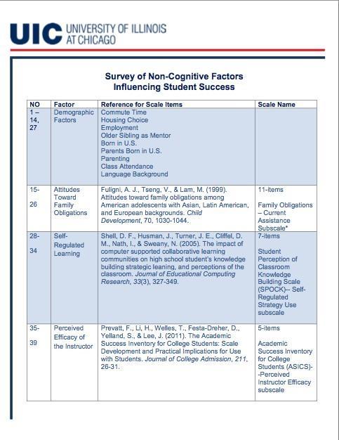
135 122

136 123

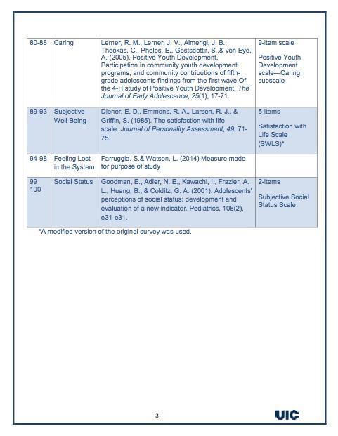
137 124